First Steps : Setting up your first case in OpenFOAM

Explore OpenFOAM with our step-by-step guide to getting your first simulation up and running. This easy-to-follow tutorial covers everything you need to know about setting up and running a basic OpenFOAM case. I break down the jargon into simple terms, explaining each step in both everyday language and plain fluid dynamics terms, so you can understand the ins and outs of your OpenFOAM case.

Embracing the wisdom of Prometheus, who once stated, ‘Big things have small beginnings,’ let’s kick off our OpenFOAM journey with a straightforward problem to understand the structure of an OpenFOAM simulation. In this instance, we’ll delve into the realm of a steady, turbulent, incompressible flow over a backward-facing step. Our simulation aims to mirror an experiment conducted in 1983 by Robert W. Pitz and John W. Daily (Reference). Their study sought to evaluate the impact of combustion on key flow field properties, including mixing layer growth, entrainment rate, and reattachment length. I will, however, stick to setting up the case.

Case setup

This specific case is available in the OpenFOAM tutorials under ~/OpenFOAM/OpenFOAM-v2312/tutorials/incompressible/simpleFoam/ or can be downloaded from here.

Once you access this case, you’ll come across three folders - 0, constant, and system. Let’s break down their roles:

• The “0” folder, a time directory, houses initial and boundary conditions crucial for the simulation. It includes specific files for various fields like velocity (“U”), pressure (“p”), and more.
• In the “constant” directory, you’ll find files detailing fluid properties, specifying turbulence modeling, and providing a comprehensive description of the domain mesh within a sub-directory named “polyMesh”.
• The “system” directory contains crucial “settings” files related to the solution process. It should feature at least three files: “controlDict” for defining simulation control parameters like start/end time and time step; “fvSchemes” for setting discretization schemes; and “fvSolution” for establishing algorithm and solver tolerances.

In simpler terms, “0” sets the boundary conditions, “constant” handles fluid properties, simulation type, and mesh details, while “system” configures the solver settings in the world of OpenFOAM.

Problem Description

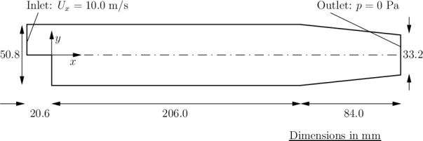
As illustrated in the above figure, we consider a 2-dimensional domain comprising a brief inlet, a backward-facing step, and a converging nozzle at the outlet. The governing equations include the continuity equation: \(\nabla \cdot u = 0\)

and the momentum or Navier-Stokes equations:

The initial conditions are set as $u = 0$ m/s and $p = 0$ Pa.

For boundary conditions, we have:

• Inlet with a fixed velocity of $u = (10, 0, 0) m/s$
• Outlet with a fixed pressure of $p = 0$ Pa
• No-slip conditions applied at the walls.

he fluid property we configure is the kinematic viscosity of air, set at $1\times 10^-5$ $m^2/s$.

To simulate the flow, I will employ the Standard k-$\varepsilon$ turbulence model and execute the simulation using the simpleFoam solver. This solver is an implementation of the SIMPLE algorithm.

0

This directory encompasses essential files containing the specified initial and boundary conditions. Since I’ve opted for the Standard k-$\varepsilon$ turbulence model, the necessary files include “U,” “p,” “k,” “epsilon,” “nut,” and “nuTilda.” If I were to choose the Standard k-$\omega$ turbulence model or k-$\omega$ SST model, I would utilize the “omega” file. While I’ve outlined the initial and boundary conditions for velocity and pressure, I haven’t explicitly mentioned them for k, epsilon, omega, nu, and nuTilda. This is because the boundary conditions for these quantities are derived from the flow’s physics.

To estimate the initial values for k, epsilon, and omega, the following formulas can be employed:

In these equations, $T_I$ represents turbulence intensity, $U_{\text{ref}}$ is the reference velocity (essentially equivalent to the inlet velocity), and $L$ denotes the characteristic length scale. The constant $C_\mu$ is assigned a value of 0.09.

constant

This folder sets up the fluid constants and the simulation type. Simple enough!!!

system

In my opinion, this folder holds high importance in the setup process. If your simulation encounters divergence or fails to run, more often than not, the culprit lies within this directory. I’ll delve into the contents of this folder extensively in my debugging article. For now, it should contain at least three crucial files: controlDict, fvSolution, and fvSchemes. Everything beyond these is either an add-on or case-specific.

• controlDict : Think of this file as equivalent to solver settings in ANSYS. It configures case controls, specifying when to halt the simulation, the time step size, intervals for writing output files, and more.
• fvSchemes : This file establishes the numerical schemes for terms in the continuity and Navier-Stokes equations. In our case, we need to define schemes for $\nabla\cdot, \nabla,$ and $\nabla^2$, representing divergence, gradient, and laplacian terms in the equation.
• fvSolution : Here, you set the solver parameters, tolerances, and algorithm preferences. In our scenario, we require a solver for p, U, k, and epsilon terms, and we’ll be using the SIMPLE algorithm.

In the controlDict file, set the time step (deltaT) to 1 for steady-state cases like this, where it serves effectively as an iteration counter. Knowing from experience that 2000 iterations are needed for reasonable convergence, set endTime to 2000. Ensure that writeInterval is sufficiently high, e.g., 100, to avoid filling the hard disk with data during runtime.

For fvSchemes, choose steadyState as the timeScheme; set gradSchemes and laplacianSchemes to default to Gauss; and use upwind for divSchemes to ensure boundedness. More details on this will be explained later.

Pay special attention to the solver settings in the fvSolution dictionary. Although the top-level simpleFoam code deals with equations for p and U only, the turbulence model solves equations for k and epsilon, necessitating tolerance settings for all equations. A tolerance of $10^{-5}$ and relTol of 0.1 are acceptable for most variables, except for p, where a tolerance of $10^{-6}$ and relTol of 0.01 are recommended. Under-relaxation of the solution is required due to the steady nature of the problem. A relaxationFactor of 0.7 is acceptable for U, k, and epsilon, but 0.3 is required for p to avoid numerical instability.

Now, you might be wondering, where does the mesh come into play? There are two methods: using a blockMesh file (in the system folder) or creating a mesh on another tool (like ANSYS ICEM or GMSH) and exporting it in .msh format. In this case, we’ll opt for the first method!!!

Running the case

Running the simulation is a straightforward process:

1. Navigate to the directory where you downloaded or copied the case file. Open a terminal at this location. Hint: When you type ls, you should see 0 constant system.
2. Activate the OpenFOAM environment. This means, source the etc/bashrc file or if you made the alias use that. For me, I will type OF2312 to source the OpenFOAM environment.
3. Generate the mesh. Type in blockMesh. Remember, OpenFOAM is case sensitive!!!
4. Run the case. Type in simpleFoam

Simple enough!!!

Post-processing

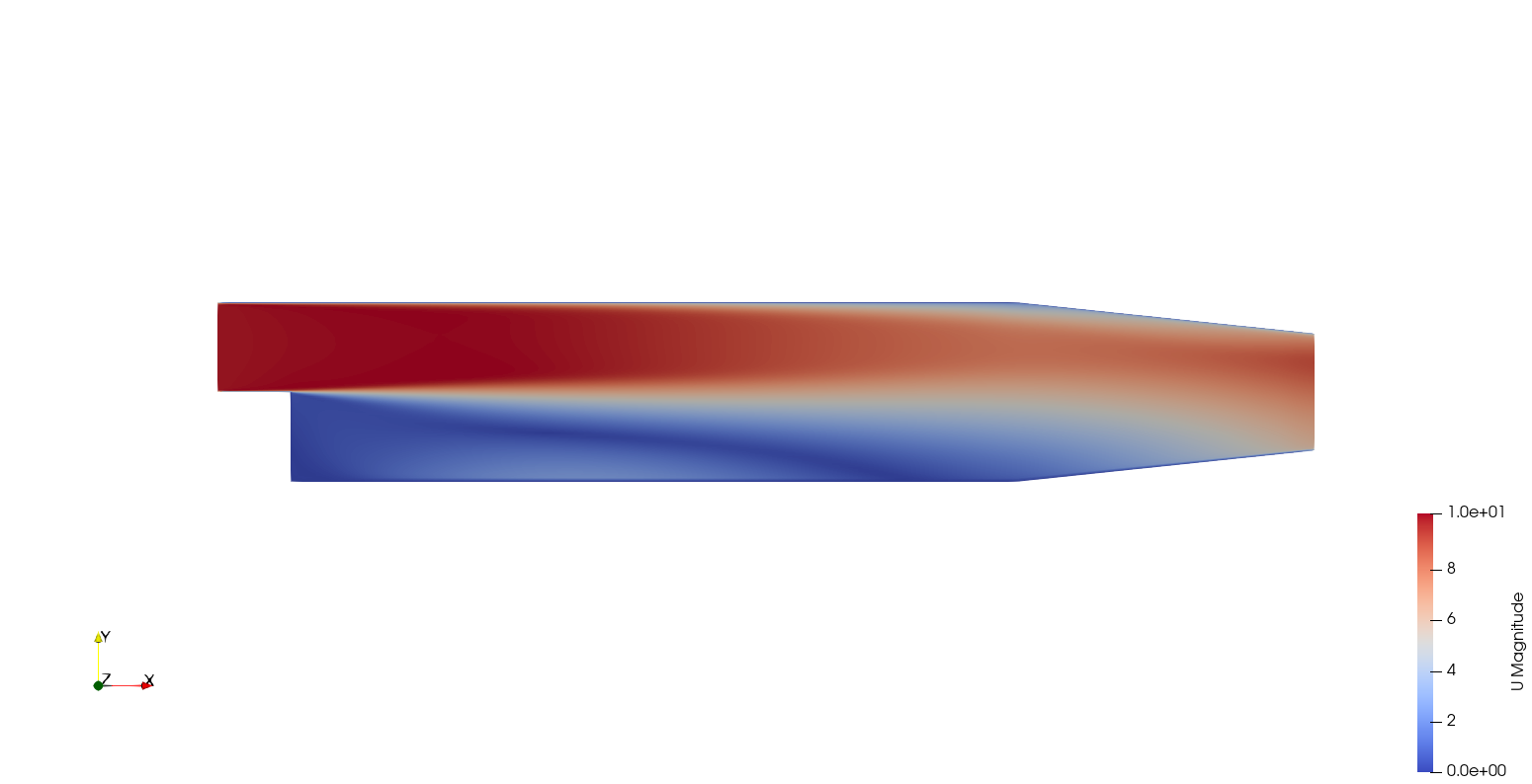
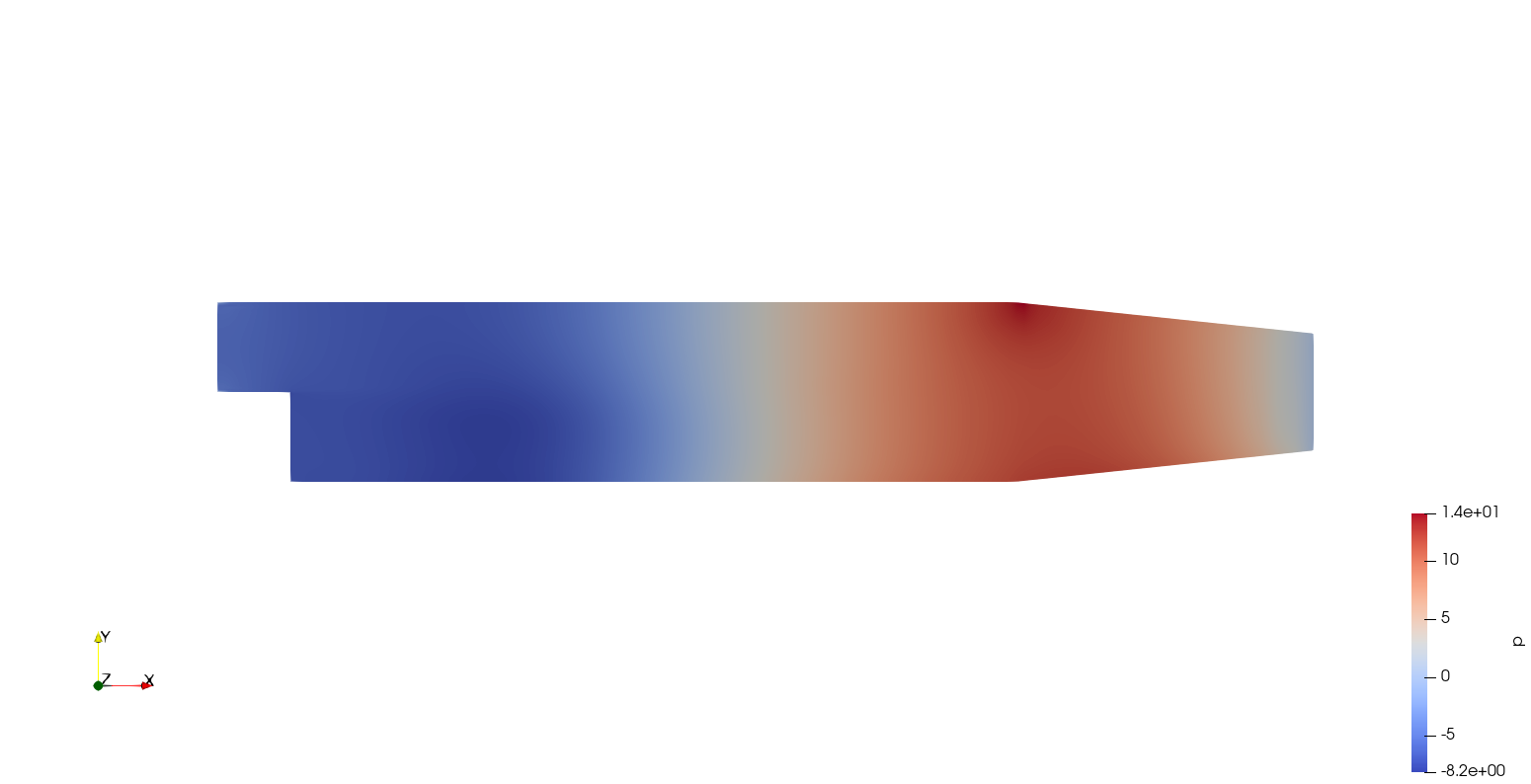
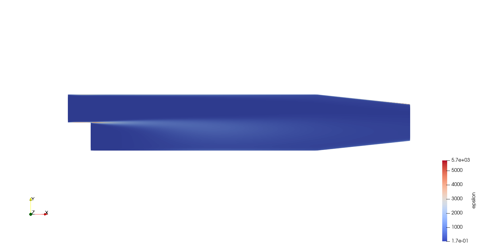
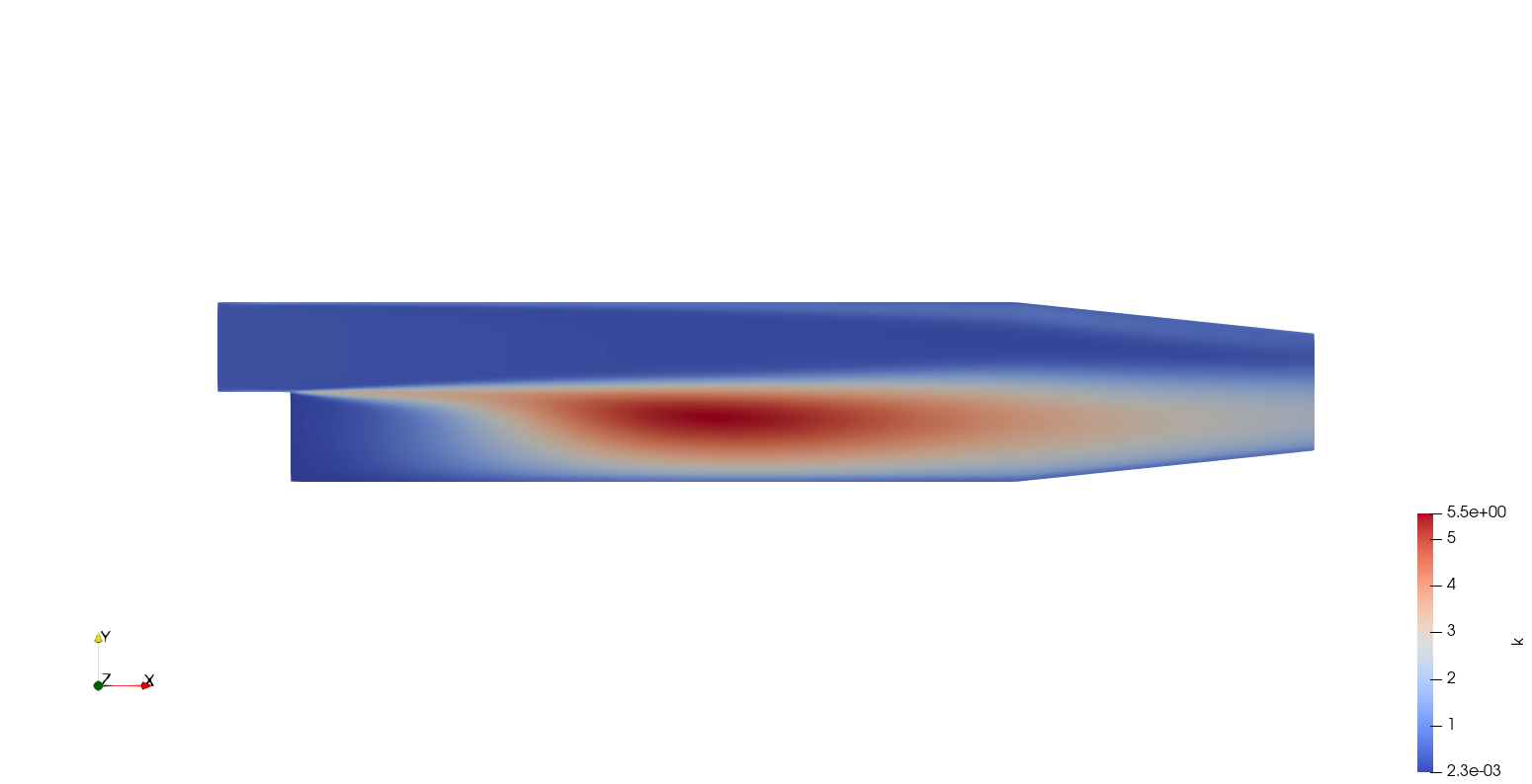
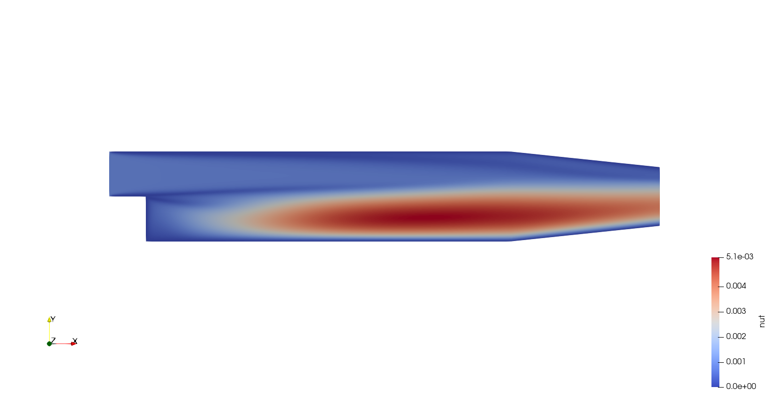
Now that the simulation is complete, let’s explore the results. To do this, simply download ParaView, a powerful visualization tool. Once installed, open your controlDict file in ParaView to visualize the results. Here are some outputs from this simulation