4 Tutorials to Rule Them All!!! (Part 1)

Introducing the complexities of setting up advanced simulations in OpenFOAM.

Setting up a tutorial case in OpenFOAM might seem like a breeze, but when it comes to tackling more intricate simulations for research purposes, the waters can quickly get murky. In this article, I will dive into the intricacies of setting up complex cases in OpenFOAM, shedding light on the challenges that arise not from geometry, but from the setup itself. Throughout this article, I’ll focus on two specific cases: the PitzDaily case and the flow around a circular cylinder. These cases serve as prime examples to illustrate the nuances of setting up various types of simulations, from steady-state to unsteady RANS-based and even Laminar or Direct Numerical Simulation (DNS). For those eager to follow along, both cases are available for download here. Additionally, I’ll be leveraging the PETSc setup introduced in a previous article, alongside the latest version of OpenFOAM, OpenFOAM-v2312, to ensure compatibility and efficiency throughout the process.

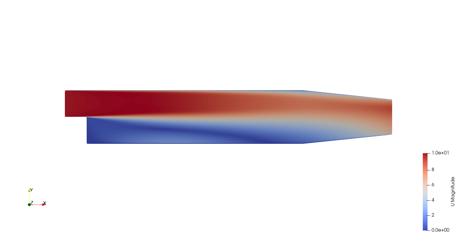
To showcase how I set up a steady-state simulation, I’ll be using the PitzDaily case labeled pitzDaily_RANS. Let’s walk through the boundary conditions necessary for this case: at the Inlet, I apply a fixed velocity of $u = (10, 0, 0) m/s$, while at the Outlet, a fixed pressure of $p = 0$ Pa is set. Additionally, I enforce No-slip conditions at the Walls. I am considering air as the fluid, with a kinematic viscosity of $1\times 10^{-5} m^2/s$. For turbulence modeling, I’ll opt for the Standard k-$\varepsilon$ model and utilize the simpleFoam solver integrated with the SIMPLE algorithm.

Now, let’s delve into key considerations when setting up a steady-state case:

0 directory

In the directory 0, it’s crucial to have the following files: “U,” “p,” “k,” “epsilon,” “nut,” and “nuTilda.”

When initializing “k” and “epsilon” (and even Omega), you can estimate their initial values using this equation:

Here, $T_I$ stands for turbulence intensity, $U_{\text{ref}}$ represents the reference velocity (essentially akin to the inlet velocity), and $L$ signifies the characteristic length scale. The constant $C_\mu$ is set to 0.09. Turbulence intensity is dependent on the Reynolds number, following the relationship $T_I = 0.16\times Re^{-1/8}$. In most cases with $Re<100000$, $T_I\approx5%$, indicating a low-turbulence scenario.

Ensure that wall functions are implemented at the wall boundary. Here’s how wall functions are incorporated:

For “k”

      Any_wall_or_Body_Surface
      {
          type            kqRWallFunction;
          value           uniform 0.375;
      }

For “epsilon”

      Any_wall_or_Body_Surface
      {
          type            epsilonWallFunction;
          value           uniform 14.855;
      }

For “omega”

      Any_wall_or_Body_Surface
      {
          type            omegaWallFunction;
          value           uniform 440.15;
      }

constant directory

In the constant directory, it’s essential to incorporate turbulence properties and configure the Standard k-$\varepsilon$ turbulence model as follows:

    simulationType      RAS;

    RAS
    {
        // Tested with kEpsilon, realizableKE, kOmega, kOmegaSST,
        // ShihQuadraticKE, LienCubicKE.
        RASModel        kEpsilon;

        turbulence      on;

        printCoeffs     on;
    }

system directory

First setup the fvSchemes file to include the a steady-state time scheme (ddtSchemes), as well as the required divSchemes. The setup of this case is as follows.

    ddtSchemes
    {
        default         steadyState;
    }

    gradSchemes
    {
        default         Gauss linear;
    }

    divSchemes
    {
        default         none;

        div(phi,U)      bounded Gauss linearUpwind grad(U);

        turbulence      bounded Gauss limitedLinear 1;
        div(phi,k)      $turbulence;
        div(phi,epsilon) $turbulence;
        div(phi,omega)  $turbulence;

        div(nonlinearStress) Gauss linear;
        div((nuEff*dev2(T(grad(U))))) Gauss linear;
    }

    laplacianSchemes
    {
        default         Gauss linear corrected;
    }

    interpolationSchemes
    {
        default         linear;
    }

    snGradSchemes
    {
        default         corrected;
    }

    wallDist
    {
        method          meshWave;
    }

Moving forward, I’ll configure the fvSolution file with the necessary solvers for this case. In my example, I’ll be utilizing the PETSc solvers. Then, I’ll set up the SIMPLE algorithm to use SIMPLE-C and establish relaxation factors as follows:

  SIMPLE
  {
      nNonOrthogonalCorrectors 0;
      consistent      yes;

      residualControl
      {
          p               1e-4;
          U               1e-6;
          "(k|epsilon|omega|f|v2)" 1e-4;
      }
  }

  relaxationFactors
  {
      equations
      {
          U               0.9; // 0.9 is more stable but 0.95 more convergent
          ".*"            0.9; // 0.9 is more stable but 0.95 more convergent
      }
  }

NOTE: In this context, the parameter nNonOrthogonalCorrectors denotes the number of non-orthogonal correctors corresponding to the non-orthogonality of the mesh. Mesh non-orthogonality is defined as the angle formed by the vector joining two adjacent cell centers across their common face and the face normal. While a square-shaped mesh element is orthogonal, a rhombus-shaped element is non-orthogonal. In real-life simulations involving complex models, numerical meshes are rarely orthogonal. Therefore, non-orthogonality correction is crucial for stability and accuracy.

A general rule-of-thumb for setting nNonOrthogonalCorrectors is as follows:

• if non-orthogonality < 70 : 0;
• if non-orthogonality > 70 : 1;
• if non-orthogonality > 80 : 2;
• if orthogonality > 85, convergence becomes challenging. (In this case, it’s advisable to improve the mesh quality.)

Now, you might wonder how to check the non-orthogonality of the mesh. You can achieve this using the checkMesh utility. When running checkMesh for your case, pay attention to the following output:

Mesh non-orthogonality Max: 5.95045 average: 1.63034
Non-orthogonality check OK.

In this example, the maximum non-orthogonality is 5.95045, suggesting that nNonOrthogonalCorrectors can be set to 0.

Lastly, let’s configure the controlDict file. For a steady-state case, the time-step or deltaT effectively serves as an iteration counter, thus set it to 1. The endTime can be a large number since a residualControl is implemented in the fvSolution. This option monitors residuals and terminates the simulation once they reach specified levels.

Running the Simulation

Based on all this information, Running the simulation is a straightforward process:

1. Navigate to the directory where you downloaded the pitzDaily_RANS case file. Open a terminal at this location. Hint: When you type ls, you should see 0 constant system.
2. Activate the OpenFOAM environment. This means, source the etc/bashrc file or if you made the alias use that. For me, I will type OF2312 to source the OpenFOAM environment.
3. Generate the mesh. Type in blockMesh. Remember, OpenFOAM is case sensitive!!!
4. Run the case. Type in simpleFoam

As I wrap up Part 1 of my exploration into advanced simulation setup in OpenFOAM, I’ve covered the essentials of preparing steady-state cases. In Part 2, I’ll delve deeper into the intricacies of setting up unsteady cases, exploring the nuances of time-stepping, turbulence modeling, and iterative solver algorithms. Stay tuned for more insights and practical tips!