4 Tutorials to Rule Them All!!! (Part 2)

10 minute read

Published: February 06, 2024

Continuing the Exploration: Advanced Simulation Setup in OpenFOAM

Welcome back to the next installment in my series on advanced simulation setup in OpenFOAM! In this sequel to my previous post, where I delved into the complexities of setting up steady-state simulations, I will now shift my focus to explore the intricacies of unsteady cases. Building upon the foundation laid in my previous discussion, I’ll navigate through the process of configuring unsteady simulations in OpenFOAM. From understanding the nuances of time stepping to implementing appropriate boundary conditions for transient behavior, I’ll cover it all. Whether you’re a seasoned OpenFOAM user or just beginning to explore the realm of computational fluid dynamics, this article promises to provide valuable insights and practical tips for mastering unsteady simulations. Let’s dive in!

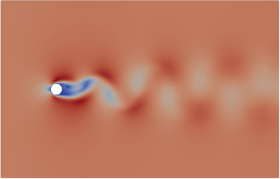
In this blog post, I’ll walk you through the setup of unsteady simulations by considering two insightful cases: Pitzdaily and the flow around a circular cylinder. You can download these cases from here, labeled as pitzDaily_RANS_unsteady, pitzDaily_Laminar, and CircularCylinder_Laminar.

laminar case in OpenFOAM is used to perform DNS. Direct Numerical Simulation (DNS) is a computational fluid dynamics (CFD) technique that provides a comprehensive solution to the Navier-Stokes equations without employing any turbulence modeling. Unlike Reynolds-Averaged Navier-Stokes (RANS) simulations, which model turbulent effects using empirical turbulence models, DNS resolves all turbulent scales explicitly. In DNS, the entire range of turbulent scales, from the largest energy-containing eddies down to the smallest dissipative scales, is resolved within the computational domain. This level of detail allows for an accurate representation of turbulent flow phenomena, making DNS particularly valuable for fundamental studies of turbulence, as well as for cases where turbulence plays a critical role in the flow behavior. However, DNS comes with significant computational costs. Resolving all turbulent scales requires a high spatial resolution, resulting in a vast number of grid points. Additionally, the small time steps necessary to capture the fast time scales of turbulence lead to lengthy simulation times, further exacerbating computational requirements. Despite its computational demands, DNS remains a powerful tool for understanding turbulence physics and validating turbulence models used in other simulation approaches like RANS or Large Eddy Simulation (LES). By providing detailed insights into flow structures and dynamics, DNS contributes to the advancement of our understanding of turbulent flows and enhances the accuracy of predictive simulations in various engineering applications.

Now, let’s delve into the essential aspects to consider when configuring an unsteady case:

constant directory

Here, I’ll start with the constant directory, where two crucial adjustments are made.

Suppose I aim to establish a RANS-based case. In this scenario, I’ll modify the turbulenceProperties file as follows:

  simulationType      RAS;

  RAS
  {
      // Tested with kEpsilon, realizableKE, kOmega, kOmegaSST,
      // ShihQuadraticKE, LienCubicKE.
      RASModel        kEpsilon;

      turbulence      on;

      printCoeffs     on;
  }

Similarly, for a laminar or Direct numerical simulation cases, I will make the following changes to the turbulenceProperties file

  simulationType  laminar;

When specifying simulationType as laminar, we essentially opt for resolving turbulence explicitly rather than utilizing turbulence models as in RANS-based simulations. It’s crucial to note that in DNS (Direct Numerical Simulation), all scales of turbulence are resolved, imposing stringent mesh requirements. Typically, DNS meshes adhere to the Kolmogorov hypothesis, where the smallest resolved scales align with the Kolmogorov length scales, denoted as $\eta = \left(\frac{\nu^3}{\varepsilon}\right)^{1/4}$.

0 directory

In setting up simulations in OpenFOAM, the contents of the 0 directory vary depending on whether we’re running laminar or RANS-based simulations.

For RANS-based simulations, following the framework established in the previous article, several crucial files are necessary: “U,” “p,” “k,” “epsilon,” “omega,” “nut,” and “nuTilda.” These files correspond to the variables involved in approximating the Navier-Stokes equations. At a minimum, “U” and “p” files are required, while the additional files are determined by the turbulence model specified in the constant/turbulenceProperties file. For instance, for the k-$\varepsilon$ family of models, “k” and “epsilon” files are needed, while for the k-$\omega$ family, “k” and “omega” files are essential. Additionally, “nut” represents turbulent viscosity, and “nuTilda” denotes kinematic turbulent viscosity, both vital for any RANS-based case.

While, in a laminar simulation, only two files are required: “U” and “p.” Since laminar simulations disregard turbulence effects, no additional variables are considered in the Navier-Stokes equations.

system directory

This is the crucial point where we draw the main distinction between a steady-state and unsteady case.

controlDict file

The time-step, represented by deltaT, holds immense significance in transient/unsteady/time-marching simulations. Before delving into its setup, let’s briefly recap the Courant–Friedrichs–Lewy (CFL) condition, a stability criterion for unsteady cases. The CFL condition dictates that the distance any information travels during the timestep length within the mesh must be lower than the distance between mesh elements. In essence, information should propagate only to immediate neighbors, not skipping mesh elements. Mathematically, CFL is expressed as: $CFL = \frac{U_{ref} \Delta t}{\Delta x}$ Here, $U_{\text{ref}}$ denotes the free-stream or bulk velocity, $\Delta t$ is the time-step, and $\Delta x$ represents the length between mesh elements (approximately the minimum element size). According to the CFL condition, $CFL\leq 1$.

Now, how do we calculate the time step, deltaT? Considering a desired $CFL\leq 0.8$ for my simulations, and with knowledge of the minimum element size ($\Delta x$) and free-stream velocity ($U_{\text{ref}}$), we estimate the time step as: $\Delta t \leq \frac{0.8\times \Delta x}{U_{ref}}$ This value is then assigned to deltaT in controlDict.

Moving on, setting up endTime is crucial. This parameter determines when the simulation should end. In transient cases, a general guideline is to set endTime to be 10 times the Through-Time. Through-Time, the time a fluid particle needs to travel between the Inlet and Outlet boundaries of the domain undisturbed, is calculated as: $Through-Time = \frac{Domain Length}{U_{ref}}$ To ensure a converged transient solution, we require at least 10 Through-Time worth of data, hence the endTime setting.

Finally, change the writeControl and writeInterval settings as required for each specific case.

fvSchemes file

Begin by configuring the fvSchemes file to incorporate an unsteady time scheme (ddtSchemes). In both laminar and RANS-based cases, the ddtSchemes are defined as follows:

  ddtSchemes
  {
      default         backward;
  }

In an unsteady case, the available options for ddtSchemes are:

default backward; : This corresponds to a second-order, implicit, backward time scheme.
default Euler; : This represents a first-order, implicit, Euler time scheme.
default CrankNicolson <coeff> : This option employs a second-order Crank-Nicolson time scheme. Here, <coeff> denotes a blending factor between full Crank-Nicolson (1) and Euler (0) schemes. The recommended choice is to use <coeff> = 0.9.

Moving on, let’s configure the divergence schemes. For a laminar simulation, the recommended divSchemes are:

  divSchemes
  {
      default         none;
      div(phi,U)      Gauss linearUpwind grad(U);
      div((nuEff*dev2(T(grad(U))))) Gauss linear;
  }

fvSolution file

The settings for solvers in fvSolution for both laminar and RANS-based cases are similar. For example, using the PETSc solvers,

    p
    {
        solver          petsc;
        preconditioner  petsc;

        petsc
        {
			
			options
            {
                ksp_type  cg;
                ksp_cg_single_reduction  true;
                mat_type mpiaij;
                pc_type  hypre;
                pc_hypre_type boomeramg;
                pc_hypre_boomeramg_max_iter "1";
                pc_hypre_boomeramg_strong_threshold "0.7";
                pc_hypre_boomeramg_grid_sweeps_up "1";
                pc_hypre_boomeramg_grid_sweeps_down "1";
                pc_hypre_boomeramg_agg_nl "2";
                pc_hypre_boomeramg_agg_num_paths "1";
                pc_hypre_boomeramg_max_levels "25";
                pc_hypre_boomeramg_coarsen_type HMIS;
                pc_hypre_boomeramg_interp_type ext+i;
                pc_hypre_boomeramg_P_max "2";
                pc_hypre_boomeramg_truncfactor "0.2";
            }


            caching
            {
                matrix
                {
                    update always;
                }

                preconditioner
                {
                    update always;
                }
            }
        }
		
        tolerance        1e-07;
        relTol           0.01;
    }

    pFinal
    {
        $p;
        relTol          0;
    }

    "(U|k|epsilon)"
    {
        solver          PBiCGStab;
		    preconditioner  DILU;
        tolerance       1e-08;
        relTol          0.01;
    }

    "(U|k|epsilon)Final"
    {
        $U;
        relTol          0;
    }

Next, we configure the iterative solver algorithm. In OpenFOAM, we have two options: PIMPLE or PISO.

The PIMPLE Algorithm combines aspects of both PISO (Pressure Implicit with Splitting of Operator) and SIMPLE (Semi-Implicit Method for Pressure-Linked Equations). Think of it as a SIMPLE algorithm applied at each time step, with outer correctors serving as iterations. Once converged, it progresses to the next time step until the solution is complete. PIMPLE tends to offer better stability, especially with large time steps where the maximum Courant number may consistently exceed 1, or when the solution is inherently unstable. It’s important to note that PISO is restricted to ${CFL}{\max}<1$, while PIMPLE’s ideal range is $5<{CFL}{\max}<1$. While PIMPLE can handle larger time steps, there’s a risk of losing crucial information, potentially leading to different results.

In OpenFOAM, we can utilize the PIMPLE Algorithm in PISO-mode by setting nOuterCorrectors 1;. With that in mind, I typically opt for the PIMPLE algorithm in PISO-mode, ensuring ${CFL}_{\max}<1$ for my simulations. Here are my iterative solver settings:

  PIMPLE
  {
      nOuterCorrectors 1;
      nCorrectors     2;
      nNonOrthogonalCorrectors 0;
  }

Why?

Setting nOuterCorrectors 1; is appropriate because I utilize PISO-mode. This configuration ensures stability in the pressure-momentum coupling.
By using nCorrectors 2;, the application (pimpleFoam) still operates in PISO mode, but with the added benefit of recalculating pressure twice. This enhances the stability of the pressure-momentum coupling, resulting in a non-diverging solution.
Finally, I set nNonOrthogonalCorrectors 0; since my mesh doesn’t exhibit significant non-orthogonality, eliminating the need for additional corrections.

Running the Simulation

Based on all this information, Running the simulation is a straightforward process:

Navigate to the directory where you downloaded pitzDaily_RANS_unsteady, pitzDaily_Laminar, and CircularCylinder_Laminar case files. Open a terminal at this location. Hint: When you type ls, you should see CircularCylinder_Laminar pitzDaily_Laminar pitzDaily_RANS_unsteady.
Navigate to any one of these cases. For example, I navigate to CircularCylinder_Laminar by cd CircularCylinder_Laminar/.
Activate the OpenFOAM environment. This means, source the etc/bashrc file or if you made the alias use that. For me, I will type OF2312 to source the OpenFOAM environment.
Run the case. Type in pimpleFoam

In conclusion, setting up unsteady simulations in OpenFOAM requires careful consideration of various parameters and algorithms. By understanding the nuances of turbulence modeling, time stepping, and iterative solver settings, we can ensure the accuracy and stability of our simulations. Whether it’s choosing between PIMPLE and PISO algorithms or fine-tuning the time-step, each decision plays a crucial role in achieving reliable results. Armed with these insights and recommendations, you’re now equipped to tackle the challenges of unsteady simulations with confidence in OpenFOAM. Happy simulating!