The OpenFOAM Game Changer: Why You Need MPI (and How to Use It)

Tired of slow OpenFOAM simulations?

Dive into the world of parallel computing with MPI and accelerate your cases to blazing speeds. This guide will equip you with the knowledge and tools to unlock the full potential of your multi-core machine or cluster, significantly reducing simulation times and boosting your research productivity. Get ready to witness the magic of parallel processing in OpenFOAM!

It’s surprising how many OpenFOAM newcomers are unaware of or ill-equipped to run simulations in parallel. This common frustration often arises when introducing OpenFOAM to fresh graduate students. Frequently asked questions like “Why is my simulation slow?” can often be answered with a simple “because you are running in Serial!” Hence, I’ve decided to address this gap by crafting an article dedicated to parallel processing in OpenFOAM. Throughout this article, I’ll utilize the flow around a circular cylinder case, downloadable from here, labeled as CircularCylinder_Laminar.

Let’s start by setting the stage. Simulating intricate real-world scenarios in OpenFOAM can be computationally demanding. Considering that most research-related simulations in OpenFOAM tackle real-world applications to some degree, learning how to leverage parallel processing becomes crucial. I’ve covered aspects of parallel processing in a previous article on setting up PETSc in OpenFOAM (Link here). Ideally, OpenFOAM simulations in research utilize High-Performance Computing (HPC) clusters, or simply put, Supercomputers. HPC clusters consist of a vast network of interconnected servers or computers known as ‘Nodes’, each equipped with components like CPU cores, memory (RAM), and disk space. While these clusters boast impressive computing power with tens of thousands of cores at your disposal, not everyone has access to them. Let’s consider reality. Not everyone has access to an HPC cluster. Sure, most universities have access to a HPC clusters and they freely (in most cases) provide them to researchers for use. For example, researchers in Canada have accees to Digital Research Alliance of Canada (formerly Compute Canada) clusters. However, access to these clusters is typically regulated by a powerful job scheduler called ‘SLURM’, ensuring fair usage among all users. In practical terms, running simulations on an HPC cluster involves preparing your case and submitting a job script to SLURM, which allocates resources and manages the execution of your simulation on compute nodes. While HPC clusters are ideal for large parallel simulations, your personal computer can serve as a valuable testing ground for smaller-scale simulations. Your PC essentially functions as a compute node, equipped with a certain number of cores, which we’ll leverage to run parallel simulations. As such, I recommend utilizing an HPC cluster for large-scale parallel simulations, reserving your personal PC for setting up or testing smaller-scale simulations.

How Many Cores?

First things first, let’s determine the number of cores your PC has.

• If you’re using macOS like me, you can check the number of cores using the terminal. Open the terminal and type in sysctl hw.physicalcpu hw.logicalcpu. This command will provide the following output:

    hw.physicalcpu: 2
    hw.logicalcpu: 4
  

• In Windows, I typically utilize the Windows Subsystem for Linux (WSL). Open your WSL terminal and type nproc. You should see something like 12. This same command should work in Ubuntu as well!

• Alternatively, for Debian-based distributions like Ubuntu, you can use the lscpu command. Running this command should yield the following output:

    Architecture:        x86_64
    CPU op-mode(s):      32-bit, 64-bit
    Byte Order:          Little Endian
    Address sizes:       43 bits physical, 48 bits virtual
    CPU(s):              64
    On-line CPU(s) list: 0-63
    Thread(s) per core:  1
    Core(s) per socket:  32
    Socket(s):           2
    NUMA node(s):        8
    Vendor ID:           AuthenticAMD
    CPU family:          23
    Model:               49
    Model name:          AMD EPYC 7532 32-Core Processor
    Stepping:            0
    CPU MHz:             2395.475
    BogoMIPS:            4790.95
    Virtualization:      AMD-V
    L1d cache:           32K
    L1i cache:           32K
    L2 cache:            512K
    L3 cache:            16384K
    NUMA node0 CPU(s):   0-7
    NUMA node1 CPU(s):   8-15
    NUMA node2 CPU(s):   16-23
    NUMA node3 CPU(s):   24-31
    NUMA node4 CPU(s):   32-39
    NUMA node5 CPU(s):   40-47
    NUMA node6 CPU(s):   48-55
    NUMA node7 CPU(s):   56-63
    ...
  

Note: To fully leverage your hardware’s capabilities, prioritize utilizing the maximum number of physical cores rather than virtual or logical cores. OpenFOAM does not optimize for logical cores or hyper-threading. Utilizing the maximum number of virtual cores may result in slower performance compared to utilizing the maximum number of physical cores. This principle also applies when running simulations on an HPC cluster.

Why Use Parallel Computing?

A straightforward answer to this lies in scalability and performance:

1. Scalability: With parallel processing, you can tackle larger problems on a simpler framework. While a single processor can only handle one task at a time, multiple processors can handle multiple tasks simultaneously.
2. Performance: Parallel processing enhances productivity and accelerates computation speed, resulting in faster execution (speed-up).

OpenFOAM Parallelization

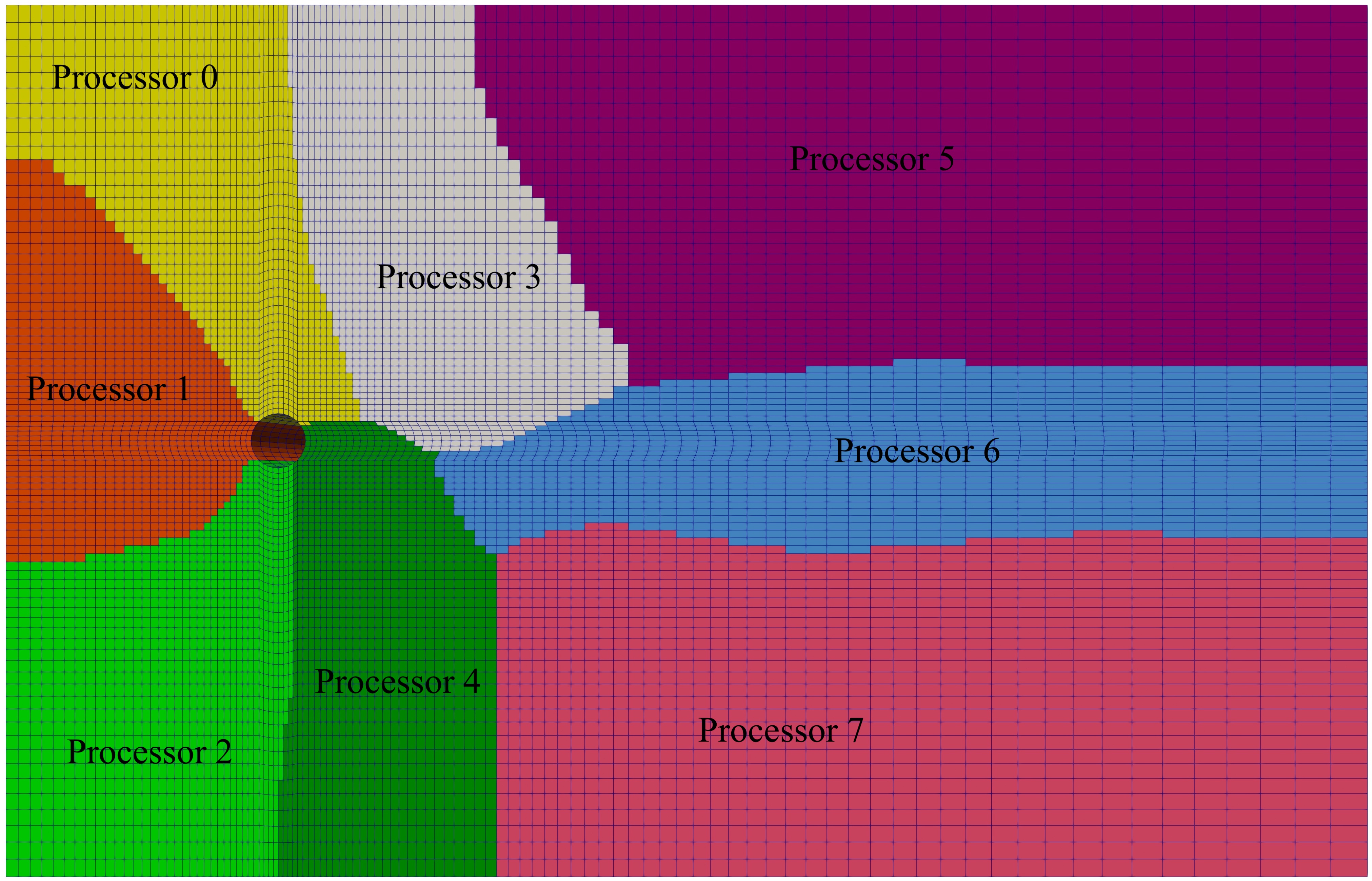
In OpenFOAM, parallel computing is achieved through domain decomposition. This process involves breaking down the geometry and associated fields (such as U, p, k, epsilon, etc.) into segments and allocating them to separate processors for computation. The parallel computation process typically includes the following steps:

1. Domain Decomposition: Breaking down the domain into smaller segments.
2. Job Distribution: Distributing the computational tasks among the available processors.
3. Parallel Simulation Execution: Running the simulation concurrently on multiple processors.
4. Result Reconstruction: Reassembling or consolidating the decomposed simulation data after completion.

In the following sections, I’ll delve into each of these steps in detail.

Decompose The Domain

The mesh and fields of your simulation are decomposed or distributed among processors using the decomposePar utility in OpenFOAM. This utility relies on parameters specified in a file called decomposeParDict, which must be present in the system directory of your simulation. Below are the dictionary entries from the decomposeParDict file in my example simulation:

/*--------------------------------*- C++ -*----------------------------------*\
| =========                 |                                                 |
| \\      /  F ield         | OpenFOAM: The Open Source CFD Toolbox           |
|  \\    /   O peration     | Version:  v1812                                 |
|   \\  /    A nd           | Web:      www.OpenFOAM.com                      |
|    \\/     M anipulation  |                                                 |
\*---------------------------------------------------------------------------*/
FoamFile
{
    version     2.0;
    format      ascii;
    class       dictionary;
    object      decomposeParDict;
}
// * * * * * * * * * * * * * * * * * * * * * * * * * * * * * * * * * * * * * //

numberOfSubdomains  24;
method          scotch;

//method          hierarchical;

hierarchicalCoeffs
{
    n           (12 2 1);
    delta       0.001; // default=0.001
    order       xyz;   // default=xzy
}
// ************************************************************************* //

Here, we specify two crucial aspects: the number of subdivisions and the decomposition method. The numberOfSubdomains parameter determines how many processors the case should be divided into. To optimize simulation performance, it’s recommended to use the maximum number of physical cores available on your machine. The number next to this entry represents the maximum number of physical cores in my machine.

The primary objective of domain decomposition is to minimize inter-processor communication and maximize simulation performance. This is where the choice of decomposition method comes into play. OpenFOAM offers four main decomposition methods:

1. simple: Divides the domain into pieces based on direction, such as nx pieces in the x-direction, ny in y, and nz in z.
2. hierarchical: Similar to simple, but allows the user to specify the order of directional splits. For instance, a decomposition of $12\times 2\times 1$ splits the domain first in the x-direction, then y, and finally z.
3. scotch: Utilizes the Scotch decomposition algorithm, minimizing the number of processor boundaries without requiring geometric input from the user. It also offers options to control decomposition strategy and weighting for machines with differing processor performance.
4. manual: Allows direct user specification of cell allocation to processors.

I recommend utilizing the scotch method. This method requires only the number of cores to use and aims to minimize processor boundaries while distributing mesh and fields.

To decompose the mesh and fields, use the decomposePar command. This utility divides the mesh and fields into the specified number of processors using the chosen method. Upon completion, it creates a set of subdirectories in the case directory, named processorN where N represents the processor number (0,1,2,..,N). Each directory contains a time directory with decomposed fields and a constant/polyMesh directory with the decomposed mesh. In my example case, the output of decomposePar will be as follows:

Decomposing mesh

Create mesh

Calculating distribution of cells
Decomposition method scotch [24] (region region0)

Finished decomposition in 6.78 s

Calculating original mesh data

Distributing cells to processors

Distributing faces to processors

Distributing points to processors

Constructing processor meshes

Processor 0
    Number of cells = 3028
    Number of points = 3813
    Number of faces shared with processor 1 = 60
    Number of faces shared with processor 2 = 88
    Number of faces shared with processor 5 = 176
    Number of faces shared with processor 22 = 175
    Number of processor patches = 4
    Number of processor faces = 499
    Number of boundary faces = 965

Processor 1
    Number of cells = 3026
    Number of points = 3858
    Number of faces shared with processor 0 = 60
    Number of faces shared with processor 2 = 216
    Number of faces shared with processor 6 = 96
    Number of faces shared with processor 16 = 112
    Number of faces shared with processor 21 = 83
    Number of faces shared with processor 22 = 166
    Number of processor patches = 6
    Number of processor faces = 733
    Number of boundary faces = 815

Processor 2
    Number of cells = 3000
    Number of points = 3789
    Number of faces shared with processor 0 = 88
    Number of faces shared with processor 1 = 216
    Number of faces shared with processor 3 = 144
    Number of faces shared with processor 5 = 128
    Number of faces shared with processor 6 = 64
    Number of processor patches = 5
    Number of processor faces = 640
    Number of boundary faces = 830

Processor 3
    Number of cells = 3016
    Number of points = 3807
    Number of faces shared with processor 2 = 144
    Number of faces shared with processor 4 = 128
    Number of faces shared with processor 5 = 144
    Number of faces shared with processor 6 = 8
    Number of faces shared with processor 9 = 208
    Number of processor patches = 5
    Number of processor faces = 632
    Number of boundary faces = 842

...

The decomposed simulation directory will appear as follows:

0           processor1   processor12  processor15  processor18  processor20  processor23  processor5  processor8
constant    processor10  processor13  processor16  processor19  processor21  processor3   processor6  processor9
processor0  processor11  processor14  processor17  processor2   processor22  processor4   processor7  system

Each processor directory will contain the fields and mesh,

processor0
├── 0
│   ├── p.gz
│   └── U.gz
└── constant
    └── polyMesh
        ├── boundary
        ├── boundaryProcAddressing.gz
        ├── cellProcAddressing.gz
        ├── cellZones.gz
        ├── faceProcAddressing.gz
        ├── faces.gz
        ├── faceZones.gz
        ├── neighbour.gz
        ├── owner.gz
        ├── pointProcAddressing.gz
        └── points.gz

Running a Parallel Simulation

To run a decomposed OpenFOAM case in parallel, we utilize openMPI, a widely used communication protocol for distributed parallel computing. Running openMPI on a local multiprocessor machine is straightforward with the following command:

mpirun -np <N_Processors> <Solver or Application> -parallel | tee log.<Solver_Name>

In this command:

• <N_Processors> specifies the number of cores being utilized.
• <Solver or Application> refers to the solver or application for the simulation.
• ... | tee log.<Solver_Name> ensures that the command output is written into a file named log.<Solver_Name>, which is considered good practice.

In my example simulations of flow around a cylinder, I use 24 cores and run the simulation with the pimpleFoam solver. Therefore, the command for my case is:

mpirun -np 24 pimpleFoam -parallel | tee log.pimpleFoam

Post Processing Parallel Simulation

Post-processing a parallel run case in OpenFOAM typically involves reconstructing the mesh and field data to recreate the complete domain and fields, which can then be post-processed as usual. I recommend this method, especially for users who prefer post-processing with Tecplot, as it can become cumbersome with a large number of time directories in parallel. Alternatively, you can directly use ParaView with the Decomposed case case-type for visualization. Additionally, for more fancy visualizations, you can post-process each segment of the decomposed domain individually.

To reconstruct the domain, simply execute:

reconstructPar

Executing reconstructPar without additional options will process all stored time directories. Specific times can be processed using options such as:

• reconstructPar -latestTime: to process the latest time only
• reconstructPar -Time N: to process time N
• reconstructPar -newTimes: to process any time directories that have not been processed previously

For the fancy visualization, manually create the file processorN.OpenFOAM (where N is the processor number) in each processor folder. Once all processorN.OpenFOAM files are created, launch ParaView and load each file. This allows visualization of the decomposed domain but provides no physical inputs into the flow.

In conclusion, parallel computing using MPI offers a powerful tool for accelerating OpenFOAM simulations, enabling users to tackle larger and more complex problems with improved efficiency. By leveraging domain decomposition and openMPI, users can fully exploit the computational resources available to them, whether on a personal machine or a high-performance computing cluster. As you embark on your parallel computing journey with OpenFOAM, remember to optimize your simulations for performance, explore post-processing techniques tailored to your needs, and never hesitate to delve deeper into the world of parallel computing for even greater efficiency gains. Happy computing!