Conquer OpenFOAM post-processing with the power of Function-objects and Python!
In the realm of OpenFOAM post-processing, navigating the intricacies becomes far simpler with the aid of a built-in utilities known as Function-objects. In this article, delve into the realm of Function-objects: discover what they are, how to effectively utilize them, and explore strategies for streamlining your post-processing tasks with the power of Python scripting.
Ever feel like wrangling your OpenFOAM data into something meaningful is an uphill battle? We’ve all been there. But fear not, the secret weapon you might be overlooking lies within OpenFOAM itself: Function-objects. These handy utilities are your key to unlocking streamlined and efficient post-processing. Forget the days of complex scripts and manual calculations. With function-objects, you can automate tasks, extract data with ease, and gain deeper insights into your simulations – all without getting tangled in code. In this article, I will delve into:
- What exactly are these function-objects? Demystifying their purpose and capabilities.
- How do you wield this power? Learn the practical steps to using function-objects in your OpenFOAM workflow.
- What magic can they unleash? Discover the diverse ways function-objects can simplify and enhance your post-processing efforts.
- Finally, sprinkle in some Python magic to supercharge your analysis even further.
In this article, I demonstrate post-processing techniques using a simulation of flow around a circular cylinder. You can access these example cases for download from here, identified as CircularCylinder_Laminar.
Lets begin!
Function Objects in OpenFOAM
OpenFOAM presents a rich array of post-processing techniques, among which function objects stand out as versatile tools. Function objects are essentially pre-built modules that empower users to monitor control points, compute forces and coefficients, perform time-averaging of fields, extract surfaces and slices, and much more—all in real-time and without requiring additional coding. These built-in utilities, defined and loaded in controlDict, enhance the capabilities of your simulations. When leveraged effectively, function objects eliminate the necessity of storing all run-time simulation data, leading to significant resource savings. Here are some additional details on what I use function objects for:
- Monitor probes : Probes are basically control points in your domain where values of certain fields are monitored over simualtion time. This feature is particularly useful for tracking critical locations or assessing the behavior of specific variables over time. For example, one can track statistical convergence using probes.
- Calculate forces and force coefficients : Users can compute forces and force coefficients acting on surfaces or boundaries within the simulation domain. This capability is essential for analyzing fluid-structure interactions, aerodynamic performance, and other engineering phenomena. For example, wind load on buildings, drag and lift forces acting on an airfoil, and so on.
- Calculate time-averaged fields : Function objects enable the calculation of time-averaged fields, providing insights into the steady-state behavior of the simulation. This is beneficial for understanding long-term trends and minimizing the influence of transient effects.
- Extract slice information : Users can extract surfaces or slices from the computational domain using function objects. This functionality is valuable for visualizing specific regions of interest or exporting data for further analysis such as Proper Orthogonal Decomposition (POD), Dynamic Mode Decomposition (DMD), and so on.
- Custom data processing : Beyond the built-in functionalities, function objects can be customized to perform user-defined data processing tasks. This flexibility allows users to tailor post-processing routines to their specific requirements, enhancing the utility of OpenFOAM for diverse applications.
How to use Function Objects ?
Function objects serve dual purposes: they can be employed during runtime within the simulation, or accessed via command-line post-processing utilities. Typically, function objects excel in runtime investigations, offering invaluable insights. To utilize function objects, each selected function must be listed within the functions sub-dictionary of the controlDict file, structured as a nested sub-dictionary, as illustrated in the following example:
...

timePrecision   8;

runTimeModifiable true;


functions
{
  <userDefinedSubDictName2>
    {
      ...
    }

  <userDefinedSubDictNameN>
  {
    ...
  }
}
Another approach to implementing function objects in controlDict is by including the file that contains them. For instance, if I define a probe function object file named probes or surfaces function objec file, I can include it in controlDict as shown below:
functions
{
  #includeFunc probes

  #includeFunc surfaces
}
Using Python for post-processing
Python serves as a powerful tool for data analysis and visualization, essential for post-processing OpenFOAM simulations. In addition to widely-used scientific modules like numpy, pandas, scipy, and matplotlib, I leverage fluidfoam. Specifically tailored for OpenFOAM, fluidfoam offers Python classes designed for straightforward post-processing of OpenFOAM data. With fluidfoam, tasks such as plotting velocity or pressure at probe points, visualizing forces and force coefficients, and plotting extracted surfaces from the surfaces function object become seamless and efficient.
Fluidfoam, a specialized Python package tailored for OpenFOAM, amplifies the post-processing capabilities by providing intuitive classes and functions. With fluidfoam, tasks that would otherwise involve intricate coding or manual processing are streamlined into simple, yet powerful operations. One notable aspect of fluidfoam is its ability to handle OpenFOAM-specific data structures seamlessly. Whether it’s accessing mesh data, field values, or function object outputs, fluidfoam simplifies the process, allowing users to focus more on analysis and less on technical intricacies. Moreover, fluidfoam facilitates the visualization of key simulation parameters, such as velocity, pressure, and turbulence fields. Through integration with matplotlib and other plotting libraries, fluidfoam enables users to generate insightful visualizations with minimal effort. In essence, fluidfoam empowers OpenFOAM users to harness the full potential of their simulation data, enabling efficient post-processing workflows and facilitating deeper insights into fluid dynamics phenomena.
To utilize the power of fluidfoam, begin by installing it via pip:
pip install fluidfoam
Once installed, fire up a Jupyter notebook and import all the essential modules:
import matplotlib.colors
import matplotlib.pyplot as plt
import numpy as np
import pandas as pd
import fluidfoam as fl
import scipy as sp

from matplotlib.colors import ListedColormap

plt.rcParams.update({'font.size' : 18, 'font.family' : 'Times New Roman', "text.usetex": True})
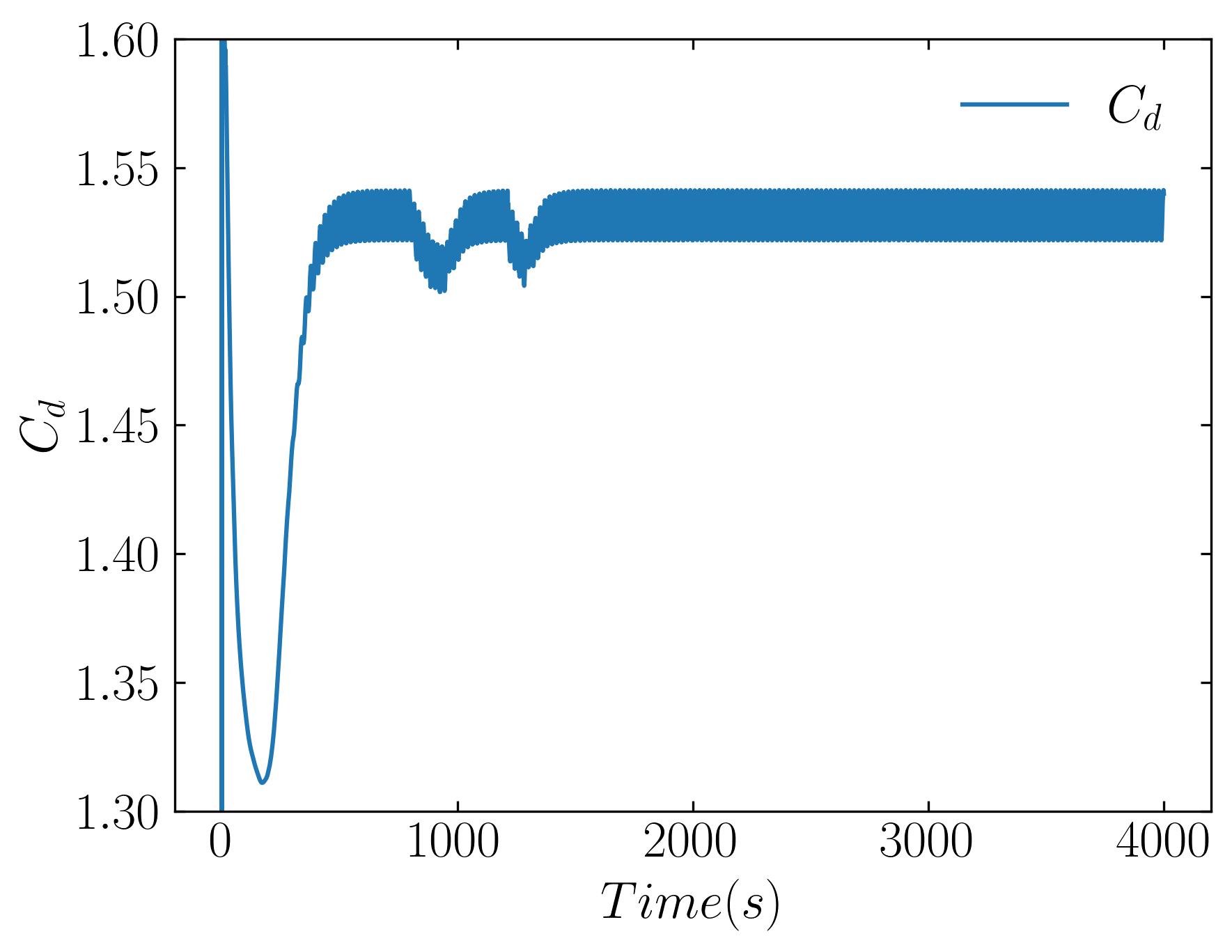
Let’s delve into an example using the readforce class from fluidfoam. This function facilitates the extraction of force coefficient data from the postProcessing/forces/coefficient file and enables plotting using matplotlib:
### Define the path to the case
Path = 'Path/To/case/postProcessing/'

### Extract force data from the coefficient file
forces = fl.readpostpro.readforce(Path, namepatch='forces',time_name='mergeTime',name='coefficient')

### Create a pandas dataframe for better column organization
### In the pressent case, the column titles are copied from the coefficient file.
df = pd.DataFrame(forces, columns=['Time','Cd','Cs','Cl','CmRoll','CmPitch','CmYaw','Cdf','Cdr','Csf','Csr','Clf','Clr'])

### Generate a plot

fig, ax = plt.subplots()

ax.plot(df['Time'], df['Cd'], label = r'$C_d$')

ax.set_ylim(1.3, 1.6)

ax.legend(loc='best', frameon = False); # or 'best', 'upper right', etc
ax.set_xlabel(r'$Time (s)$')
ax.set_ylabel(r'$C_d$')
ax.xaxis.set_tick_params(direction='in', which='both')
ax.yaxis.set_tick_params(direction='in', which='both')
ax.xaxis.set_ticks_position('both')
ax.yaxis.set_ticks_position('both')

# plt.savefig(Path + 'Drag.jpeg', dpi = 300, bbox_inches = 'tight')

plt.show()
This script will produce the specified plot.
Similarly, fluidfoam enables the extraction of probe data effortlessly:
### for velocity at probes
probes_loc, time, u = fl.readpostpro.readprobes(Path ,probes_name='probes',time_name='mergeTime',name='U')

### for pressure at probes
probes_loc, time, p = fl.readpostpro.readprobes(Path ,probes_name='probes',time_name='mergeTime',name='p')
With fluidfoam’s simplicity and efficiency, post-processing OpenFOAM simulations becomes a breeze. Check out fluidfoam at fluidfoam.readthedocs.io.
Examples of Function-Objects
Here are some examples of function objects that I commonly use in my simulations.
In conclusion, mastering function objects and leveraging tools like fluidfoam can significantly streamline your OpenFOAM post-processing workflow. By harnessing the power of Python and its scientific libraries, you can extract valuable insights from your simulation data with ease and precision. Whether you’re plotting force coefficients, analyzing probe data, or visualizing flow fields, these techniques empower you to take your simulations to new heights. So, dive in, experiment, and unlock the full potential of your OpenFOAM simulations. Happy computing!
Enjoy Reading This Article?
Here are some more articles you might like to read next: