The Final Frontier: Conquering OpenFOAM Post-Processing with Command-Line Power
Ready to take your OpenFOAM post-processing skills to the next level? This guide completes our post-processing triology, delving into conventional post-processing: extracting and analyzing data after your simulation finishes. Unlock the power of command-line techniques and discover how to effortlessly visualize your data using Python. Learn to extract specific data points, analyze results, and create compelling visuals to gain deeper insights from your OpenFOAM simulations.
Wrapping up our exploration of various post-processing techniques in OpenFOAM, this final installment delves into command-line post-processing. In prior articles, I’ve delved into run-time post-processing using function objects within OpenFOAM and explored simplifying post-processing with Python [Links here]. Run-time post-processing offers users flexibility by providing access to all time steps during simulation, not just data written out. It allows monitoring of processed data during simulation, offering immediate results at simulation’s end. However, what if you forget to include the correct function objects before running simulations? Or if, like many novice researchers, you’re unsure what post-processing you’ll need beforehand? What if you actually want to ‘post’ process your data? This is where command-line post-processing proves invaluable.
In the traditional sense, post-processing, as the term implies, involves data manipulation conducted after a simulation concludes. This allows users to analyze data using available results like time directories and fields once the simulation has run its course. There are two primary methods for post-processing in OpenFOAM: conventional post-processing via the postProcess utility and solver-run post-processing through <solver> -postProcess utility. Both methods leverage the functionality embedded in OpenFOAM’s function object framework. The conventional postProcess utility applies any function object to the data within time directories, while the solver-run utility executes function objects specified in the controlDict file.
To illustrate command-line post-processing techniques, let’s consider the flow around a circular cylinder as a case study. You can download the simulation files from here, labeled as Cylinder_Run. This case has already been executed, providing one time directory. We’ll utilize this case to accomplish three post-processing tasks:
- Extracting data along multiple lines from the simulation.
- Computing fluctuating velocity and vorticity.
- Visualizing the simulation results by extracting a cross-section (surface/slice) through the domain.
Without further ado, let’s dive in.
Command-line post-processing in OpenFOAM
Exploring the two command-line post-processing methods mentioned earlier, let’s delve into how they are executed.
Standard postProcess utility:
The standard postProcess utility in OpenFOAM is executed with the following command:
postProcess -func <functions>
Solver-run post-processing utility:
For instance, with pimpleFoam, the solver-run post-processing utility is invoked using:
pimpleFoam -postProcess -func <functions>
You can find a comprehensive list of available function objects for both of these functionalities in the $FOAM_ETC/caseDicts/postProcessing directory within your OpenFOAM installation. Here, you’ll find a myriad of options to suit your post-processing needs, including:
postProcessing/
├── fields
├── flowRate
├── forces
├── graphs
├── lagrangian
├── minMax
├── numerical
├── pressure
├── probes
├── solvers
│   └── scalarTransport
├── surfaceFieldValue
└── visualization
Extracting data along lines
Let’s delve into practical learning by extracting data along a line specified between two points from the simulation. To begin, we’ll create a file named sampleDict. This file will house the function object necessary for post-processing. Since we’re interested in sampling a line, we’ll generate a file named MultipleLines within the system directory. This file will contain the function object for sets, which is utilized to sample lines. In this scenario, we aim to extract velocity, pressure, mean velocity, mean pressure, and prime-squared mean velocity data along three lines defined by 1000 points. Additionally, we’ll format the data in .csv format, including the coordinates of the extracted data. Below is an illustrative example of such a file:
/*--------------------------------*- C++ -*----------------------------------*\
  =========                 |
  \\      /  F ield         | OpenFOAM: The Open Source CFD Toolbox
   \\    /   O peration     |
    \\  /    A nd           | Web:      www.OpenFOAM.com
     \\/     M anipulation  |
-------------------------------------------------------------------------------
Description
    Writes graph data for specified fields along a line, specified by start
    and end points.

\*---------------------------------------------------------------------------*/


// Sampling and I/O settings
#includeEtc "caseDicts/postProcessing/graphs/sampleDict.cfg"

type            sets;
libs            ("libsampling.so");

writeControl    writeTime;

interpolationScheme cellPoint;

setFormat   csv;

setConfig
{
    type    uniform;
    axis    xyz;  // x, y, z, xyz
	nPoints	1000;
}

sets
(
    line1
    {
        $setConfig;
        start   (0 0 0);
		end     (1.8 0 0);
    }

	line2
    {
        $setConfig;
        start (0.4 0.8 0);
        end   (0.4 -0.8 0);
    }

	line3
    {
        $setConfig;
        start (0.8 0.8 0);
        end   (0.8 -0.8 0);
    }
);

fields  (U p UMean pMean UPrime2Mean);

// ************************************************************************* //
Now, let’s proceed to extract the data using the postProcess utility with the command:
postProcess -func MultipleLines
Executing this command will generate a folder within the postProcessing directory containing the extracted fields stored in .csv files. The directory structure will resemble the following:
MultipleLines/
└── 4996.9
    ├── line1_p_pMean_U_UMean_UPrime2Mean.csv
    ├── line2_p_pMean_U_UMean_UPrime2Mean.csv
    └── line3_p_pMean_U_UMean_UPrime2Mean.csv
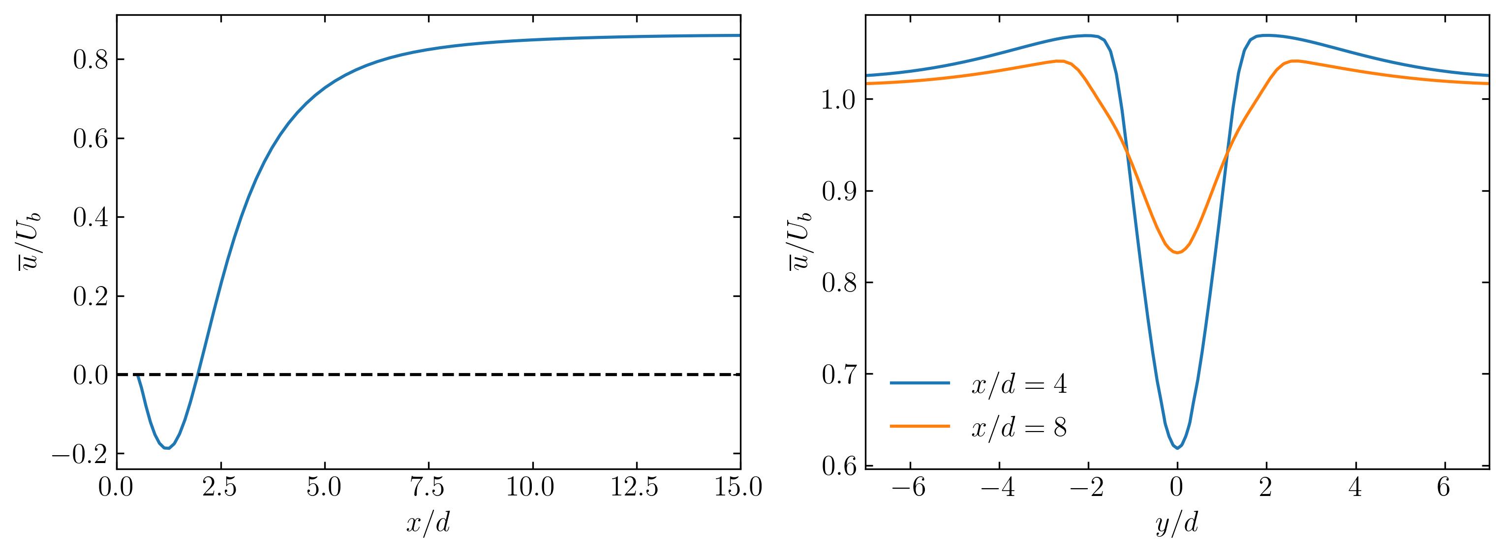
These CSV files contain the sampled data along the specified lines. To visualize this data, one can easily plot it using Python. Below, I provide an example of plotting the mean axial velocity along the three lines.
For plotting the data, you can utilize a Python script, preferably within a Jupyter Notebook, as demonstrated below:
### import modules

import matplotlib.colors
import matplotlib.pyplot as plt
import numpy as np
import pandas as pd
import fluidfoam as fl
import scipy as sp
import os

%matplotlib inline

plt.rcParams.update({'font.size' : 14, 'font.family' : 'Times New Roman', "text.usetex": True})

### set paths
Path = 'E:/4_Tutorials/Cylinder_DNS/postProcessing/'
save_path = 'E:/4_Tutorials/Cylinder_DNS/'
MultipleLinesData = 'MultipleLines/4996.9/' ## specify latestTime folder

### get the list of files
Files = os.listdir(Path + MultipleLinesData)

### extract data from csv files using pandas
Line1 = pd.read_csv(Path + MultipleLinesData + Files[0])
Line2 = pd.read_csv(Path + MultipleLinesData + Files[1])
Line3 = pd.read_csv(Path + MultipleLinesData + Files[2])

### plot mean axial velocity profiles

d = 0.1
Ub = 0.015

fig, axes = plt.subplots(1,2, figsize = (12,4))

ax = axes[0]

ax.plot(Line1.x/d, Line1.UMean_0/Ub)
ax.axhline(0, color = 'k', linestyle = '--')

ax.set_ylabel(r'$\overline{u}/U_b$')
ax.set_xlabel(r'$x/d$')

ax.xaxis.set_tick_params(direction='in', which='both')
ax.yaxis.set_tick_params(direction='in', which='both')
ax.xaxis.set_ticks_position('both')
ax.yaxis.set_ticks_position('both')

ax.set_xlim(0, 15)

ax = axes[1]

ax.plot(Line2.y/d, Line2.UMean_0/Ub, label = r'$x/d = 4$')
ax.plot(Line3.y/d, Line3.UMean_0/Ub, label = r'$x/d = 8$')

ax.set_ylabel(r'$\overline{u}/U_b$')
ax.set_xlabel(r'$y/d$')

ax.xaxis.set_tick_params(direction='in', which='both')
ax.yaxis.set_tick_params(direction='in', which='both')
ax.xaxis.set_ticks_position('both')
ax.yaxis.set_ticks_position('both')

ax.legend(loc = 'best', frameon = False) # or 'best', 'upper right', etc

ax.set_xlim(-7, 7)

plt.savefig(save_path + 'Velocity_Plots.jpeg', dpi = 300, bbox_inches = 'tight')

plt.show()
Why opt for this method? This method of extracting data is a staple in my daily workflow, especially during extensive simulations where regular check-ins on field development are essential. Using the MultipleLine dictionary post-simulation allows me to swiftly extract the required data without relying on Paraview or VisIt. By simply augmenting this dictionary with as many lines as necessary, I efficiently extract the desired data. When you’re clear on the data needed and its source, this utility proves to be the quickest route from extraction to visualization.
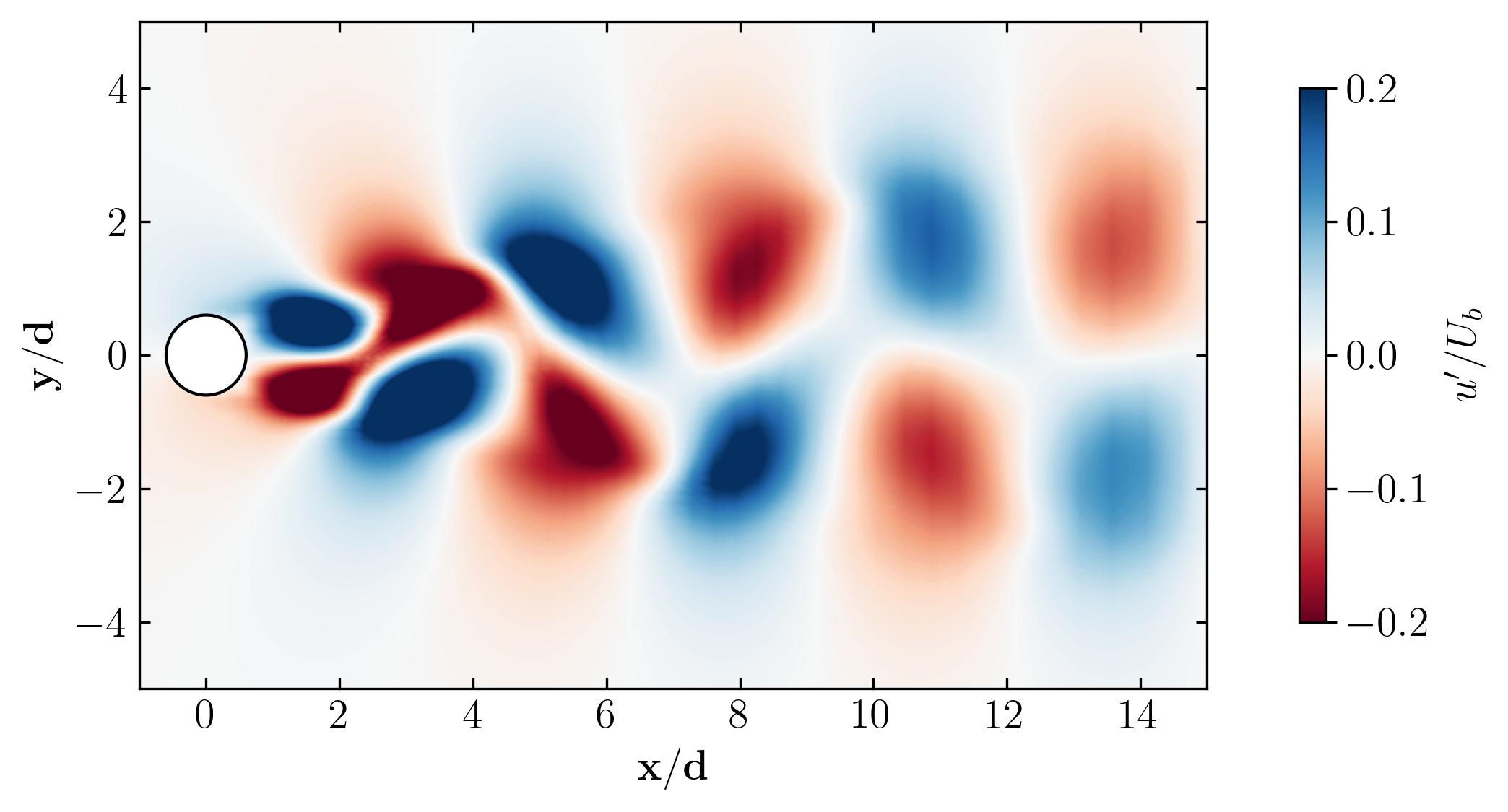
Computing fluctuating field and vorticity
In the previous example, we explored extracting existing data along specified lines. Now, let’s delve into calculating entirely new fields. In this instance, we’ll compute two fields: the fluctuating velocity field and the vorticity field. To achieve this, we’ll leverage the solver-run post-processing utility. Let’s begin with computing the vorticity, which can be accomplished with the following command:
pimpleFoam -postProcess -func vorticity -field "(U)"
Upon execution, this command computes the vorticity using the velocity field (duh!!!) and writes the field out in the time directory under the name vorticity.
Now, let’s move on to calculating the fluctuating velocity fields. This is achieved by subtracting the mean velocity from the instantaneous velocity. However, attempting to perform this operation using the solver-run post-processing command pimpleFoam -postProcess -func "subtract(U, UMean)" may lead to a common error. The error typically encountered is as follows:
--> FOAM FATAL ERROR: (openfoam-2312)

    failed lookup of UMean (objectRegistry region0)
    available objects of type volVectorField:
3(U_0 U U_0_0)


    From const Type& Foam::objectRegistry::lookupObject(const Foam::word&, bool) const [with Type = Foam::GeometricField<Foam::Vector<double>, Foam::fvPatchField, Foam::volMesh>]
    in file /home/goswami/OpenFOAM/OpenFOAM-v2312/src/OpenFOAM/lnInclude/objectRegistryTemplates.C at line 628.

FOAM exiting
Here’s a quick debugging tip in OpenFOAM: Always read the error message carefully. In this case, the error indicates that the UMean field is not available in the objectRegistry, listing the available fields as 3(U_0 U U_0_0). Essentially, this means that the UMean field isn’t accessible to the objectRegistry because it’s generated by a function object during runtime. The solver-based post-processing command will only work in case of fields available in the objectRegistry. To inspect what is available in the objectRegistry, you can use the following command:
Available objects in database:

24
(
MRFProperties
U
U_0
U_0_0
boundary
cellZones
data
faceZones
faces
fvOptions
fvSchemes
fvSolution
neighbour
nu
owner
p
phi
phi_0
phi_0_0
pointZones
points
solutionControl
transportProperties
turbulenceProperties
)
This scenario arises whenever a field is generated by a function object during runtime. In such cases, the standard postProcess utility should be used, like so:
postProcess -func "subtract(U, UMean)"
Executing this command will generate a file named subtract(U,UMean) within the time directories.
Why opt for this method? For the sake of streamlined data processing. By incorporating these commands into a script, particularly useful when working on a computing cluster, you can efficiently obtain ready-to-post-process fields. This eliminates the need to generate these fields manually in software like Paraview or Tecplot, simplifying your workflow significantly.
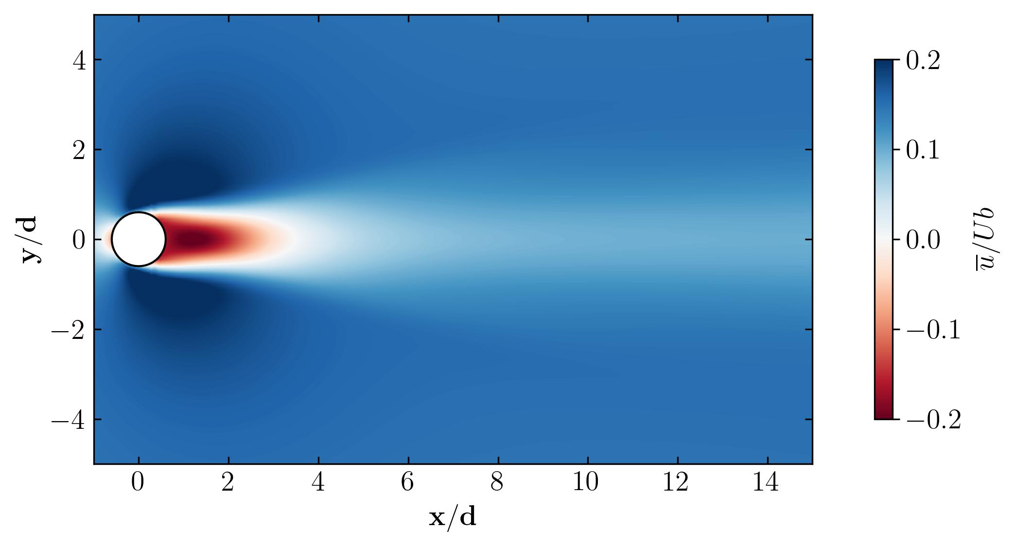
Extracting surfaces and visualizing the field
Now that we’ve computed the vorticity and fluctuating velocity fields, let’s proceed to visualize them in Python. To achieve this, I’ll utilize the surfaces function object executed through the command-line. The surfaces function object samples field values on surfaces and writes the results to a file using the selected output file format. To begin, we’ll create a file named surfaces in the system directory. This file will contain the surfaces function object, extracting a z-normal surface at the span-wise center of the domain. Below is an example of such a file:
/*--------------------------------*- C++ -*----------------------------------*\
  =========                 |
  \\      /  F ield         | OpenFOAM: The Open Source CFD Toolbox
   \\    /   O peration     |
    \\  /    A nd           | Web:      www.OpenFOAM.com
     \\/     M anipulation  |
-------------------------------------------------------------------------------
Description
    Writes out values of fields from cells nearest to specified locations.

\*---------------------------------------------------------------------------*/
surfaces
{
    type            surfaces;
    libs            ("libsampling.so");
    writeControl   	timeStep;
    writeInterval   10;

    surfaceFormat   vtk;

	formatOptions
	{
		vtk
		{
			legacy true;
			format ascii;
		}
	}

    fields          (p U UMean vorticity subtract(U, UMean));

    interpolationScheme cellPoint;

    surfaces
    {
        zNormal
        {
            type        cuttingPlane;
            point       (0 0 0);
            normal      (0 0 1);
            interpolate true;
        }
    };
};
// ************************************************************************* //
Now, let’s proceed to extract the data using the postProcess utility with the command:
postProcess -func surfaces
Executing this command will generate a file named surfaces within the postProcessing directory, containing the surface field in a vtk file, as shown below:
surfaces/
└── 4996.9
    └── zNormal.vtk
This vtk file can be readily opened in Paraview or VisIt for visualization. However, the focus of this article is to visualize these fields in Python using the PyVista module. PyVista is a powerful tool for 3D data visualization, serving as an interface for the Visualization Toolkit (VTK). With PyVista, one can easily read and extract data from a vtk file. For this demonstration, I highly recommend using a Jupyter Notebook for ease of navigation between sets of codes. Let’s start by importing the module, in addition to the ones before:
import pyvista as pv
Let’s set the path variables to the case and the required files:
### set paths
Path = 'E:/4_Tutorials/Cylinder_DNS/postProcessing/'
save_path = 'E:/4_Tutorials/Cylinder_DNS/'
surfaces = 'surfaces/4996.9/' ## specify latestTime folder

### extract files
Files = os.listdir(Path + surfaces)
Now, read the vtk file zNormal.vtk using the PyVista module and extract the coordinate data:
Data = pv.read(Path + surfaces + Files[0])
grid = Data.points
x = grid[:,0]
y = grid[:,1]
z = grid[:,2]
rows, columns = np.shape(grid)
print('rows = ', rows, 'columns = ', columns)
By printing out the array names from this Data variable, one can simply list all the available fields within this vtk file:
print(Data.array_names)
### Output
### ['TimeValue', 'p', 'U', 'UMean', 'fluctuations', 'vorticity']
At this point, let’s extract the point data and print out their sizes to find the number of components within a field. Fields such as velocity, vorticity, and fluctuations will have three components:
vorticity = Data.point_data['vorticity']
fluctuations = Data.point_data['fluctuations']
velocity = Data.point_data['U']
pressure = Data.point_data['p']

print(vorticity.shape, fluctuations.shape, velocity.shape, pressure.shape)

### Output
### (9260, 3) (9260, 3) (9260, 3) (9260,)
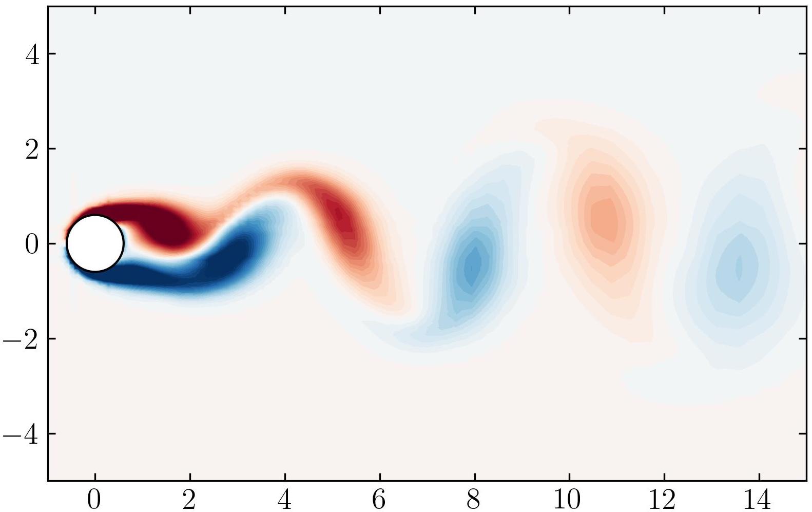
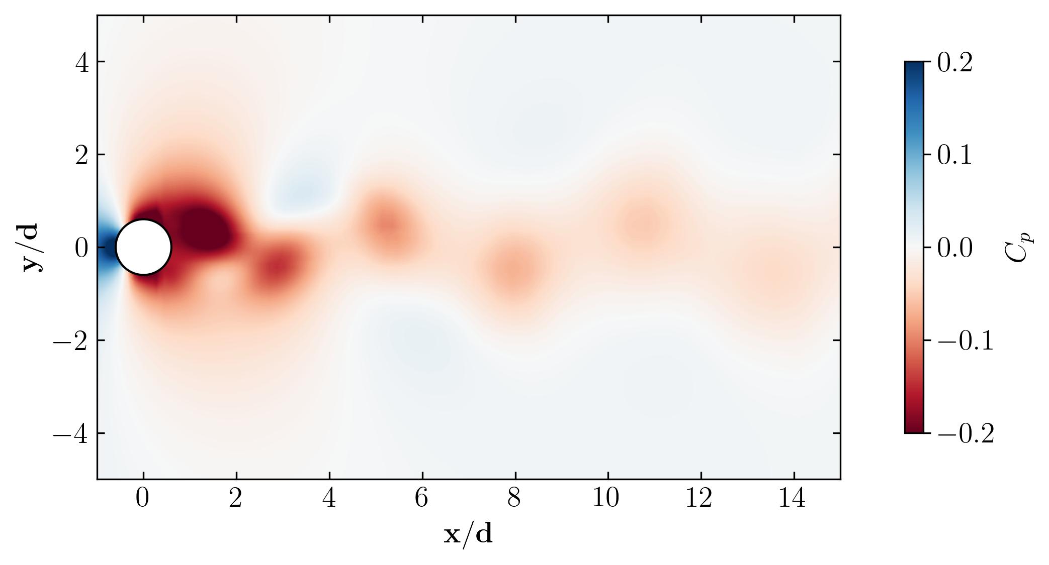
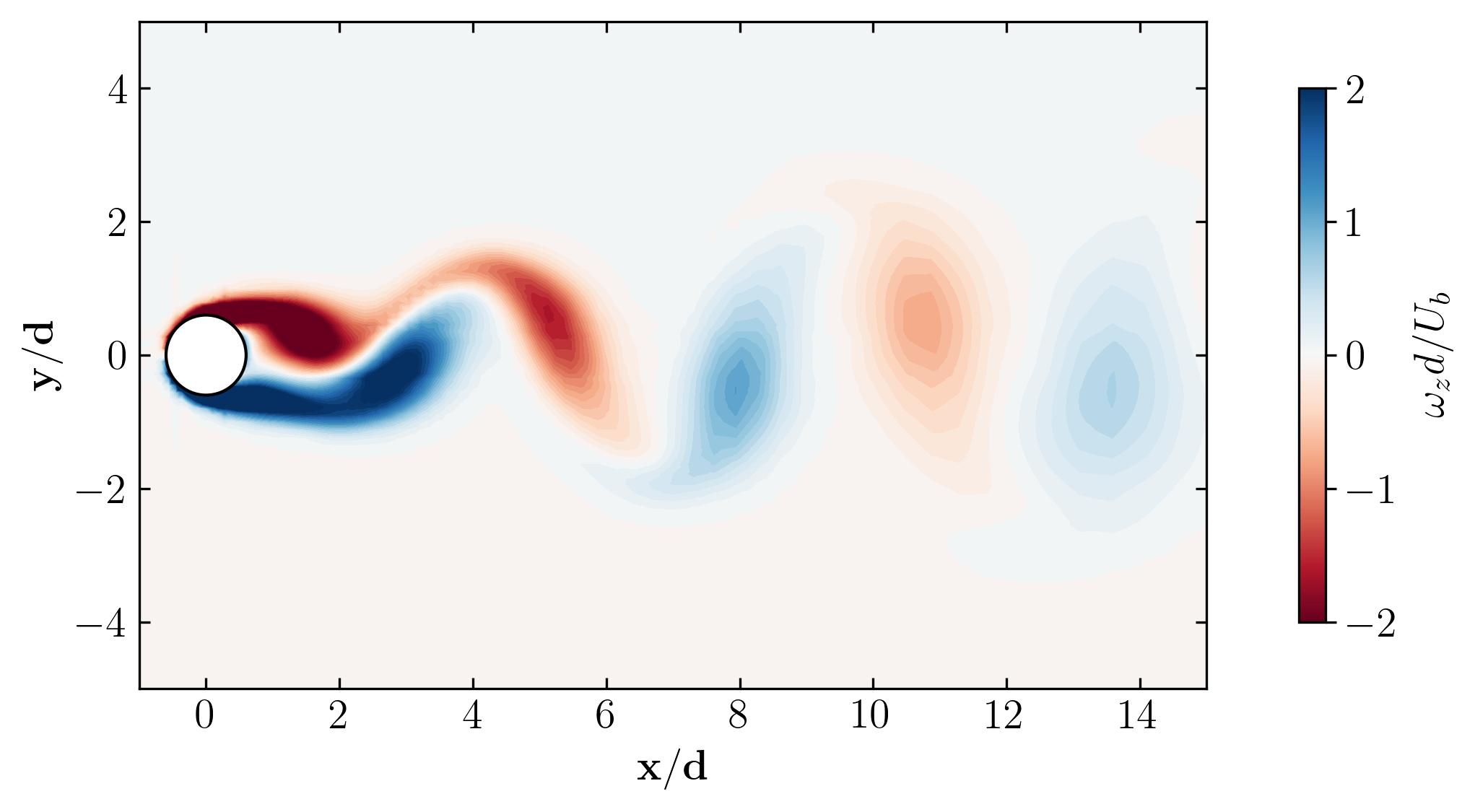
Finally, let’s plot the extracted data using a tricontourf plot in matplotlib.
# circle1 = plt.Circle((0, 0), 0.05, ec='k', color='grey')
Circle1 = plt.Circle((0, 0), 0.6, ec='k', color='white')
# Rect2 = plt.Rectangle((0, 0), 1, 1, ec='k', color='grey')

fig, ax = plt.subplots(figsize=(11, 4))

p = ax.tricontourf(x/0.1, y/0.1, vorticity[:,2]*(d/Ub), levels = 501, vmin=-2, vmax=2, cmap = 'RdBu')
# cb = fig.colorbar(p, ax=ax, shrink=0.8)
m = plt.cm.ScalarMappable(cmap='RdBu')
m.set_array(vorticity[:,2])
m.set_clim(-2, 2)
plt.colorbar(m, ax=ax, shrink=0.8)
# ax.quiver(x/0.01, y/0.01, U[:,0]/3.75, U[:,1]/3.75, scale=15)

ax.add_patch(Circle1)
# ax.axvline(0.1856, c='w', ls='--', lw=1)
# ax.axvline(0.1856/2, c='w', ls='--', lw=1)
ax.xaxis.set_tick_params(direction='in', which='both')
ax.yaxis.set_tick_params(direction='in', which='both')
ax.xaxis.set_ticks_position('both')
ax.yaxis.set_ticks_position('both')
# ax.set_xscale('log')
ax.set_xlim(-1, 15)
ax.set_ylim(-5, 5)
# ax.set_box_aspect(4/11)
ax.set_aspect('equal')

ax.set_xlabel(r'$\bf x/d$')
ax.set_ylabel(r'$\bf y/d$')
# ax.set_title(r'$\bf x/d = 1$')

# plt.savefig(save_path + 'Mode2.jpeg', dpi = 300, bbox_inches = 'tight')

plt.show()
Behold, the figures generated by the script:
As a final note, let’s explore the versatility of Python. Beyond static visualizations, Python empowers you to create dynamic presentations, including animations. Imagine capturing the mesmerizing dance of vortex shedding in motion. With Python, the possibilities are endless. So why not give it a try? Dive in, experiment, and unleash the full potential of Python for your fluid dynamics simulations. The world of dynamic visualizations awaits!
Why opt for this method? Once again, simplicity reigns supreme. With Python and PyVista, visualizing the extracted surfaces is a breeze. But why opt for this method? Let me count the ways.
-
Ease of Use: Python combined with PyVista simplifies the visualization process, making it accessible to users of all skill levels.
-
Scriptability: Harness the power of scripting to automate visualization tasks, saving time and effort in the long run.
-
Customization: Tailor your plots to perfection with Python’s extensive libraries and matplotlib’s flexible customization options.
-
Interactivity: Dive deeper into your data with interactive jupyter notebooks, allowing for real-time exploration and analysis.
In essence, this method offers not just visualization, but a seamless and dynamic experience, enhancing your understanding and insights into your data.
And with that, we wrap up the trilogy of articles on OpenFOAM post-processing. It’s important to remember that post-processing should be simple and painless – a no-brainer, if you will. After all, the goal isn’t just to generate pretty pictures. In fluid mechanics and CFD, the true aim is to articulate your insights clearly and concisely. What you visualize is only as valuable as your ability to explain the underlying mechanics of physical processes.
So, as you delve into the realm of computational fluid dynamics, keep in mind that CFD stands for Computational Fluid Dynamics, not Colorful Fluid Dynamics. Focus on understanding and communicating the essence of your simulations.
Happy computing!!!
Enjoy Reading This Article?
Here are some more articles you might like to read next: