Dive Deeper with fluidfoam: Advanced Techniques for Extracting & Analyzing OpenFOAM Data
Craving deeper insights from your OpenFOAM simulations? Explore the wonders of Python post-processing with fluidfoam. Learn how to effortlessly extract and visualize key data points like force coefficients and velocity probes, turning complex data into clear and interpretable results. This guide equips you with the tools to unlock the true potential of your simulations and gain valuable knowledge from every run.

In my previous article, we explored how Python is indespensible for data-analysis in OpenFOAM simulations, and briefly looked into fluidfoam, a specialized Python package tailored for OpenFOAM post-processing. Fluidfoam simplifies complex tasks like plotting velocity and pressure distributions, handling OpenFOAM-specific data structures seamlessly, and enabling insightful visualizations with minimal effort. It represents a significant advancement in post-processing workflows, empowering users to extract deeper insights from their simulation data. Here is my previous article for reference here.
In my previous article, I introduced the basics of fluidfoam, a specialized Python package designed for post-processing in OpenFOAM simulations. In this installment, I’m excited to delve deeper into advanced post-processing techniques using fluidfoam. Specifically, we’ll explore three key aspects:
- Extracting and plotting velocity at probe points.
- Extracting and plotting force coefficients.
- Plotting the power spectral density of velocity at probe points and force coefficients.
These advanced techniques will enable us to gain deeper insights into our OpenFOAM simulations and enhance our understanding of fluid dynamics phenomena. So without further ado, let’s dive in!
Ready the case
I’ll be demonstrating these post-processing techniques using a simulated flow around a circular cylinder as an example. You can access the example cases for download from here, identified as CircularCylinder_Laminar. While I’ll be using this specific case for illustration, the techniques showcased are applicable to any simulation provided there is sufficient data available. For this demonstration, the CircularCylinder_Laminar case is initially run until 4000 seconds (endTime) to ensure fully-developed flow. Subsequently, the simulation is extended for another 1000 seconds with the inclusion of additional function objects in the controlDict under the functions sub-dictionary. Specifically, I incorporate function objects probes and forces into the simulation setup, as depicted below:
functions
{
    #includeFunc probes

    forces
    {
        type            forceCoeffs;
        libs ( "libforces.so" );

        writeControl   timeStep;
        writeInterval  1;

        patches         ( "PRISM" );

        rho             rhoInf;
        log             true;
        rhoInf          1.225;
        liftDir         (0 1 0);
        dragDir         (1 0 0);
        //sideDir         (0 0 1);
        CofR            (0 0 0);
        pitchAxis       (0 0 1);
        magUInf         0.015;
        lRef            0.1;
        Aref            0.0628;
    }

}
Here, I’m including the probes file below for reference. In situations where you need to monitor multiple probe locations, such as hundreds of points, it’s advisable to maintain a separate file named probes within your system folder and then include this file in the functions section of your controlDict file. This approach helps maintain clarity and organization in your simulation setup. Here is an example of probes file,
/*--------------------------------*- C++ -*----------------------------------*\
  =========                 |
  \\      /  F ield         | OpenFOAM: The Open Source CFD Toolbox
   \\    /   O peration     |
    \\  /    A nd           | Web:      www.OpenFOAM.com
     \\/     M anipulation  |
-------------------------------------------------------------------------------
Description
    Writes out values of fields from cells nearest to specified locations.

\*---------------------------------------------------------------------------*/
probes
{
    type            probes;
    libs            ("libsampling.so");

    // Name of the directory for probe data
    name            probes;

    // Write at same frequency as fields
    writeControl    timeStep;
    writeInterval   1;

fields (
        p
        U
       );

probeLocations
(

	(0.01 0 0)
	(0.02 0 0)
	(0.03 0 0)
	(0.04 0 0)
	(0.05 0 0)

);
    // Optional: filter out points that haven't been found. Default
    //           is to include them (with value -VGREAT)
    includeOutOfBounds  true;
}
// ************************************************************************* //
Running the simulations for the last 1000 seconds with function objects will generate a directory named postProcessing within your case directory. This postProcessing directory will contain the data derived from the function objects, structured as illustrated below:
postProcessing
├── forces
│   └── 3996.9
│       └── coefficient.dat
└── probes
    └── 3996.9
        ├── U
        └── p
Understanding Probe Data Extraction
To extract and plot the probes, we’ll utilize the fluidfoam and matplotlib packages in Python. Let’s start by importing the necessary modules. While I typically prefer using Jupyter Notebook (.ipynb), these steps are also applicable for a Python script (.py).
import matplotlib.colors
import matplotlib.pyplot as plt
import numpy as np
import pandas as pd
import fluidfoam as fl
import scipy as sp

%matplotlib inline

plt.rcParams.update({'font.size' : 14, 'font.family' : 'Times New Roman', "text.usetex": True})
Set a path to your case,
### Path to CircularCylinder_Laminar/postProcessing directory
Path = 'E:/4_Tutorials/CircularCylinder_Laminar/postProcessing'
### Path where to save the figures
save_path = 'E:/4_Tutorials/CircularCylinder_Laminar/'
Let’s extract the velocity probes. We’ll accomplish this using the readprobes function from within fluidfoam. With this function, we have the flexibility to extract probe data from all folders within postProcessing using the mergeTime option, or we can solely extract data from the last-run time directory using the latestTime option. In the following example, I’ll extract the probes using the latestTime option:
### Read Probes of u
probes_locU, timeU, u = fl.readpostpro.readprobes(Path ,probes_name='probes',time_name='latestTime',name='u')
This function extracts three main components: probe locations, the corresponding time stamps for each probe, and the velocity components at these probe locations. Probe locations are presented as a numpy array and can be non-dimensionalized as follows:
### Probe Locations
Locations = probes_locU/0.1
print(Locations)
I typically recommend visualizing these probe locations in a tabular format for better comprehension. Since we’re dealing with only 5 probes in this example, I’ll print out these locations here. They appear in the format (x, y, z):
[[0.1 0.  0. ]
 [0.2 0.  0. ]
 [0.3 0.  0. ]
 [0.4 0.  0. ]]
The velocity at these probe locations is extracted in the format: u[probes list (all or index), Probe location (from Probes_locU), velocity components (ux, uy, uz) = (0,1,2)]. This means the first index of u represents the list of all velocities, the second index signifies the index-location of the probe, and the third index represents the velocity components as (ux, uy, uz) = (0, 1, 2).
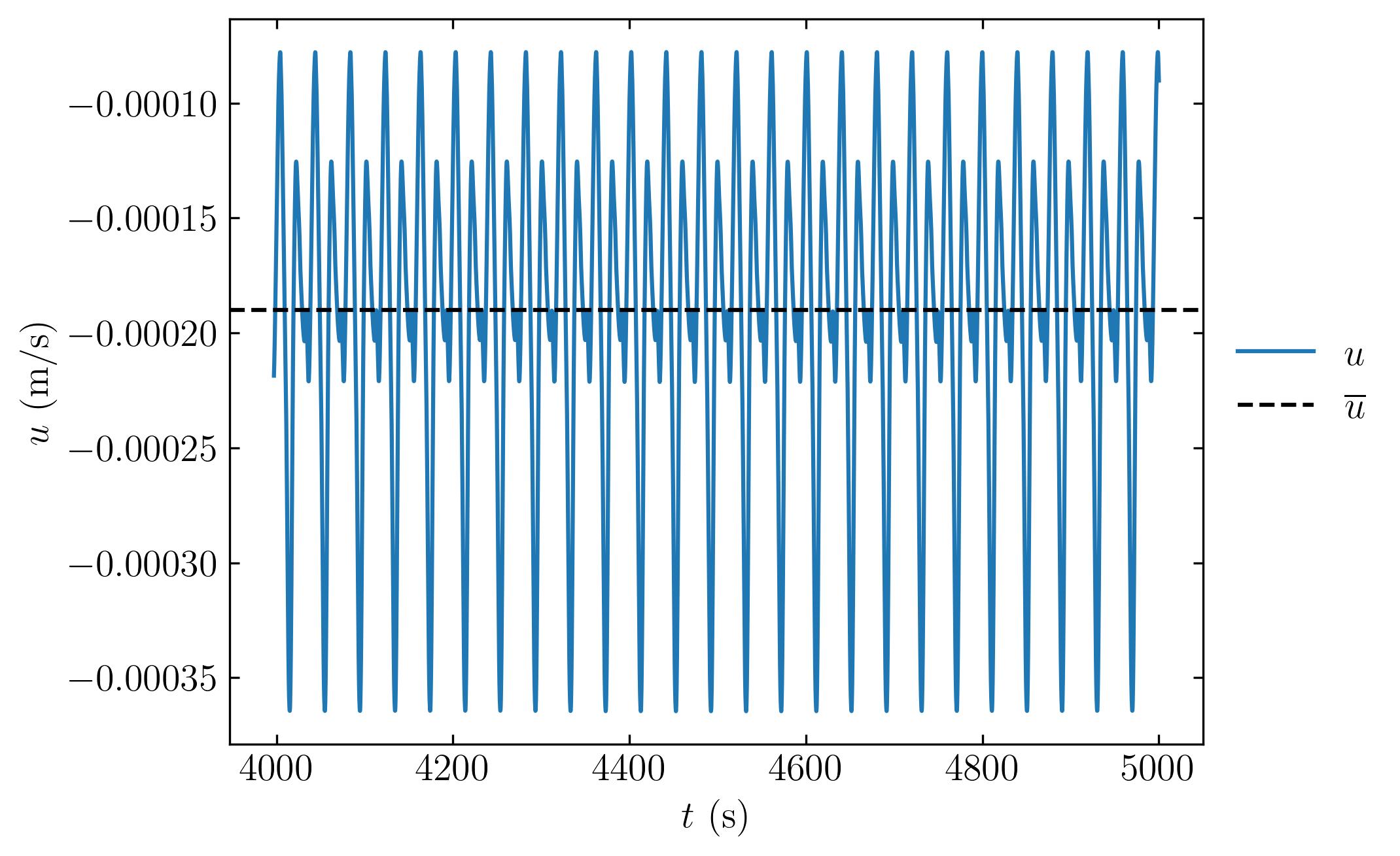
You can plot the velocity at any probe location using the following method:
fig, ax = plt.subplots()
ax.plot(timeU, u[:, 4, 0], label=r'$u$')
ax.axhline(np.mean(u[:, 4, 0]), color='k', linestyle='--', label=r'$\overline{u}$')

ax.set_ylabel(r'$u$ (m/s)')
ax.set_xlabel(r'$t$ (s)')

ax.xaxis.set_tick_params(direction='in', which='both')
ax.yaxis.set_tick_params(direction='in', which='both')
ax.xaxis.set_ticks_position('both')
ax.yaxis.set_ticks_position('both')

ax.legend(loc = 'center left', frameon = False, bbox_to_anchor = (1, 0.5))


plt.savefig(save_path + 'probeVelocity.jpeg', dpi = 300, bbox_inches = 'tight')

plt.show()
Understanding Force Coefficient Extraction
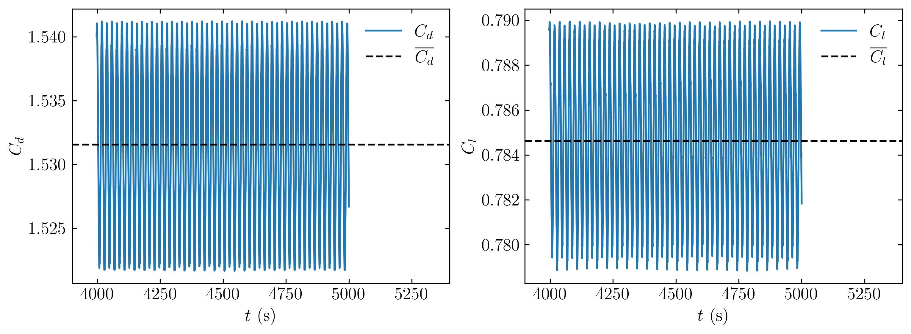
In the same way, we can plot the force coefficients by,
### extract the force coefficients
forces_Coefficients = fl.readpostpro.readforce(Path,namepatch='forces',time_name='mergeTime',name='coefficient')
### Create a pandas dataframe for better column organization
### In the pressent case, the column titles are copied from the coefficient file.
df = pd.DataFrame(forces_Coefficients, columns=['Time','Cd','Cs','Cl','CmRoll','CmPitch','CmYaw','Cdf','Cdr','Csf','Csr','Clf','Clr'])

fig, axes = plt.subplots(1,2, figsize = (12,4))

ax = axes[0]

ax.plot(df.Time, df.Cd, label=r'$C_d$')
ax.axhline(np.mean(df.Cd), color='k', linestyle='--', label=r'$\overline{C_d}$')

ax.set_ylabel(r'$C_d$')
ax.set_xlabel(r'$t$ (s)')

ax.xaxis.set_tick_params(direction='in', which='both')
ax.yaxis.set_tick_params(direction='in', which='both')
ax.xaxis.set_ticks_position('both')
ax.yaxis.set_ticks_position('both')

ax.legend(loc = 'upper right', frameon = False) # or 'best', 'upper right', etc

ax.set_xlim(3900, 5400)

ax = axes[1]

ax.plot(df.Time, df.Cl, label=r'$C_l$')
ax.axhline(np.mean(df.Cl), color='k', linestyle='--', label=r'$\overline{C_l}$')

ax.set_ylabel(r'$C_l$')
ax.set_xlabel(r'$t$ (s)')

ax.xaxis.set_tick_params(direction='in', which='both')
ax.yaxis.set_tick_params(direction='in', which='both')
ax.xaxis.set_ticks_position('both')
ax.yaxis.set_ticks_position('both')

ax.legend(loc = 'upper right', frameon = False) # or 'best', 'upper right', etc

ax.set_xlim(3900, 5400)

plt.savefig(save_path + 'Forces.jpeg', dpi = 300, bbox_inches = 'tight')

plt.show()
Power spectral density of velocity and force coefficient
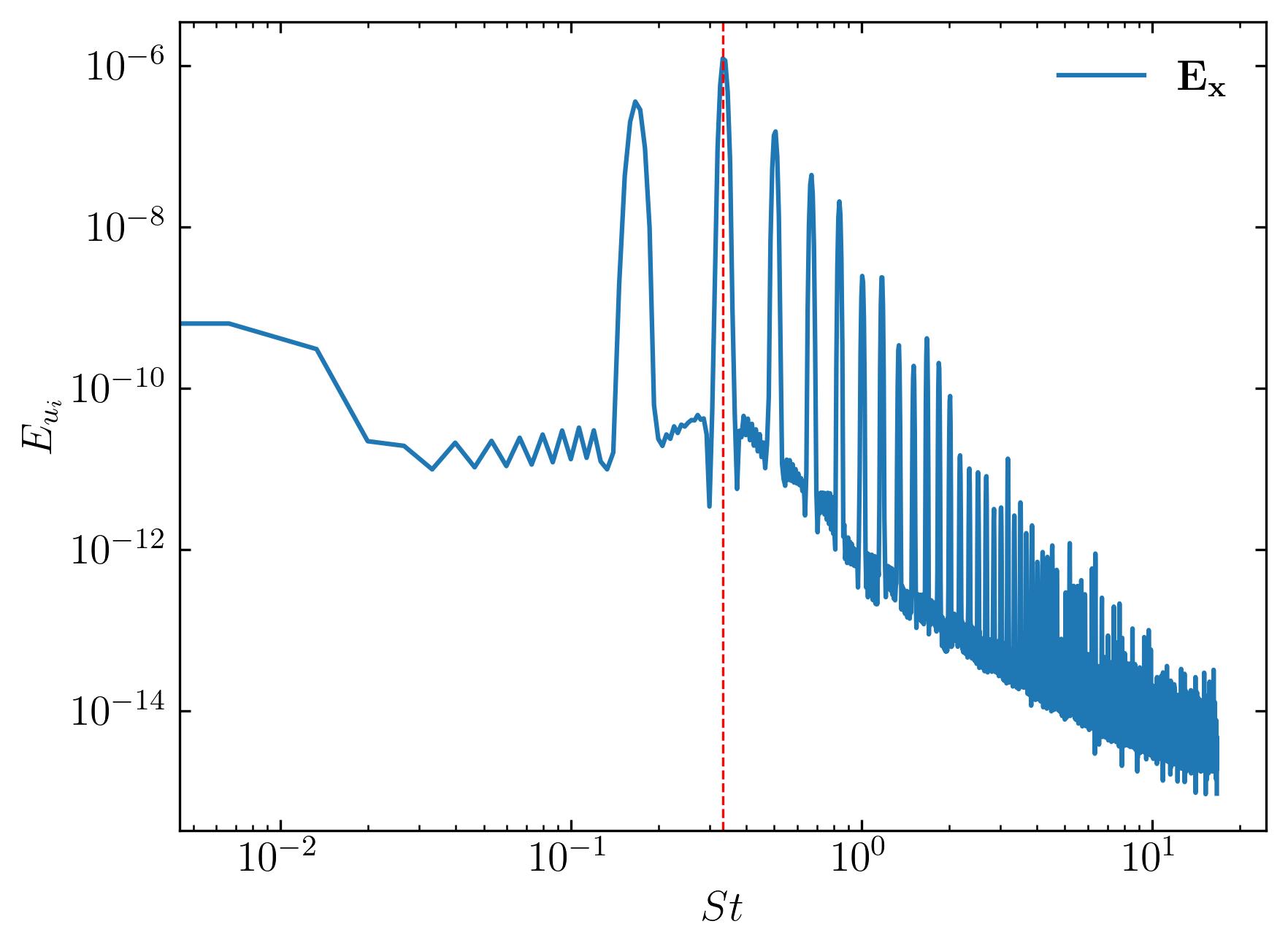
The power spectral density characterizes the power contained within a signal across different frequencies. In wake studies conducted using Computational Fluid Dynamics (CFD), power spectral density is employed to identify dominant frequencies within the flow, often used to estimate the Strouhal number - a non-dimensional frequency parameter. The Strouhal number (St) is computed as St = f*L/U, where f represents the vortex shedding frequency, L denotes the characteristic length scale, and U signifies the free-stream velocity. Generating the power spectrum of velocity at specific probe locations involves:
### FFT

### Constants
d = 0.1
Ub = 0.015
dt = 0.2
fs = 1/dt

Signal1 = u[:, 4, 0]

### PSD using welch
f1, Eu1 = sp.signal.welch(Signal1, fs, nfft = len(Signal1), nperseg=len(Signal1)/2, window='hamming')
St1 = f1*d/Ub

fig, ax = plt.subplots()

ax.loglog(St1, Eu1, label = (r'$\bf E_x$'))

### Mark and print the dominant frequency
xmax = St1[np.argmax(Eu1*f1/(Ub**2))]
print("Strouhal Number = ", xmax)
ax.axvline(xmax, c='r', ls='--', lw=0.8)

ax.legend(loc='best', frameon = False); # or 'best', 'upper right', etc
ax.set_xlabel(r'$St$')
ax.set_ylabel(r'$E_{u_i}$')
ax.xaxis.set_tick_params(direction='in', which='both')
ax.yaxis.set_tick_params(direction='in', which='both')
ax.xaxis.set_ticks_position('both')
ax.yaxis.set_ticks_position('both')

plt.savefig(save_path + 'Power.jpeg', dpi = 300, bbox_inches = 'tight')

plt.show()
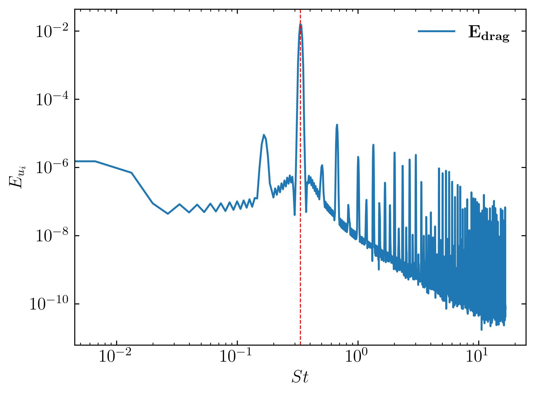
To compute the power spectrum of the coefficient of drag, simply substitute the signal with df.Cd, as demonstrated below:
### FFT

### Constants
d = 0.1
Ub = 0.015
dt = 0.2
fs = 1/dt

Signal1 = df.Cd

### PSD using welch
f1, Eu1 = sp.signal.welch(Signal1, fs, nfft = len(Signal1), nperseg=len(Signal1)/2, window='hamming')
St1 = f1*d/Ub

fig, ax = plt.subplots()

ax.loglog(St1, Eu1, label = (r'$\bf E_{drag}$'))

### Mark and print the dominant frequency
xmax = St1[np.argmax(Eu1*f1/(Ub**2))]
print("Strouhal Number = ", xmax)
ax.axvline(xmax, c='r', ls='--', lw=0.8)

ax.legend(loc='best', frameon = False); # or 'best', 'upper right', etc
ax.set_xlabel(r'$St$')
ax.set_ylabel(r'$E_{u_i}$')
ax.xaxis.set_tick_params(direction='in', which='both')
ax.yaxis.set_tick_params(direction='in', which='both')
ax.xaxis.set_ticks_position('both')
ax.yaxis.set_ticks_position('both')

plt.savefig(save_path + 'PowerDrag.jpeg', dpi = 300, bbox_inches = 'tight')

plt.show()
In conclusion, mastering advanced post-processing techniques such as extracting and analyzing velocity probes, plotting force coefficients, and examining power spectral density is essential for gaining deeper insights into fluid dynamics simulations. Through the utilization of tools like fluidfoam and Python libraries such as matplotlib, we can efficiently extract and visualize crucial data points, enabling us to better understand the behavior of fluid flows in complex systems. By harnessing these techniques, researchers and engineers can enhance their ability to interpret simulation results, leading to more accurate predictions and informed decision-making in various fields, from aerospace engineering to renewable energy applications. As computational fluid dynamics continues to advance, proficiency in post-processing methodologies will remain paramount for unlocking new discoveries and pushing the boundaries of fluid dynamics research and development. Happy computing!
Enjoy Reading This Article?
Here are some more articles you might like to read next: