Beyond Pretty Pictures: Trusting Your Results with CFD Verification and Validation (Part 2)

Now that we’ve established the importance of Verification and Validation (V&V) in CFD, buckle up! Part 2 of this series takes us on a deeper dive. We’ll explore practical best practices specifically designed for CFD research. Get ready to uncover essential strategies, tools, and methodologies to ensure the accuracy and reliability of your simulations, propelling your CFD work to the next level.

‘Cleverly Forged Data’ or ‘Computational Fluid Dynamics’ – the ultimate dilemma that resonates with every CFD researcher.

In a previous discussion, we delved into the intriguing world of Verification and Validation, unraveling the complexities through a simple yet profound exploration of the steady-state one-dimensional convection-diffusion equation. We peeled back the layers to reveal how meticulous grid sensitivity analysis bolsters the integrity of our numerical solutions, setting the stage for robust and precise simulations. Meanwhile, the validation process illuminated the daunting challenge of aligning our virtual realities with real-world experimental data, particularly within the enigmatic realms of the Navier-Stokes equations, where analytical solutions remain elusive. Despite the inherent challenges, innovative strategies offer promising avenues to navigate the verification and validation maze. While verification scrutinizes the correctness of our numerical methods, validation zeroes in on the accuracy of our simulations in mirroring real-world phenomena.

Link to Part 1

In this installment, we embark on a journey to uncover essential insights for conducting dependable and credible CFD analysis. From selecting the appropriate simulation model to scrutinizing grid independence, and from fine-tuning time-step parameters for transient simulations to validating the numerical setup and flow physics – we’ll explore each aspect meticulously.

To ensure dependable and credible CFD analysis, several key steps are imperative:

1. Select appropriate model for simulation.
2. Grid independence.
3. Time-step independence for transient simulations.
4. Check the mass and continuity errors.
5. Boundary condition sensitivity analysis / Domain independence.
6. Validation of numerical setup or flow physics.

Join me as we dissect these crucial components, offering invaluable tips and strategies from the perspective of a seasoned CFD researcher. Together, let’s pave the way towards trustworthy and reliable CFD analysis, one step at a time.

Selection of appropriate model

The selection of an appropriate simulation model is paramount in CFD, as it significantly impacts both the computational resources required and the accuracy of the results obtained. Thorough research is essential to identify the suitable models for handling various phenomena such as turbulence, multiphase flow, and species transport, tailored to the specific case at hand.

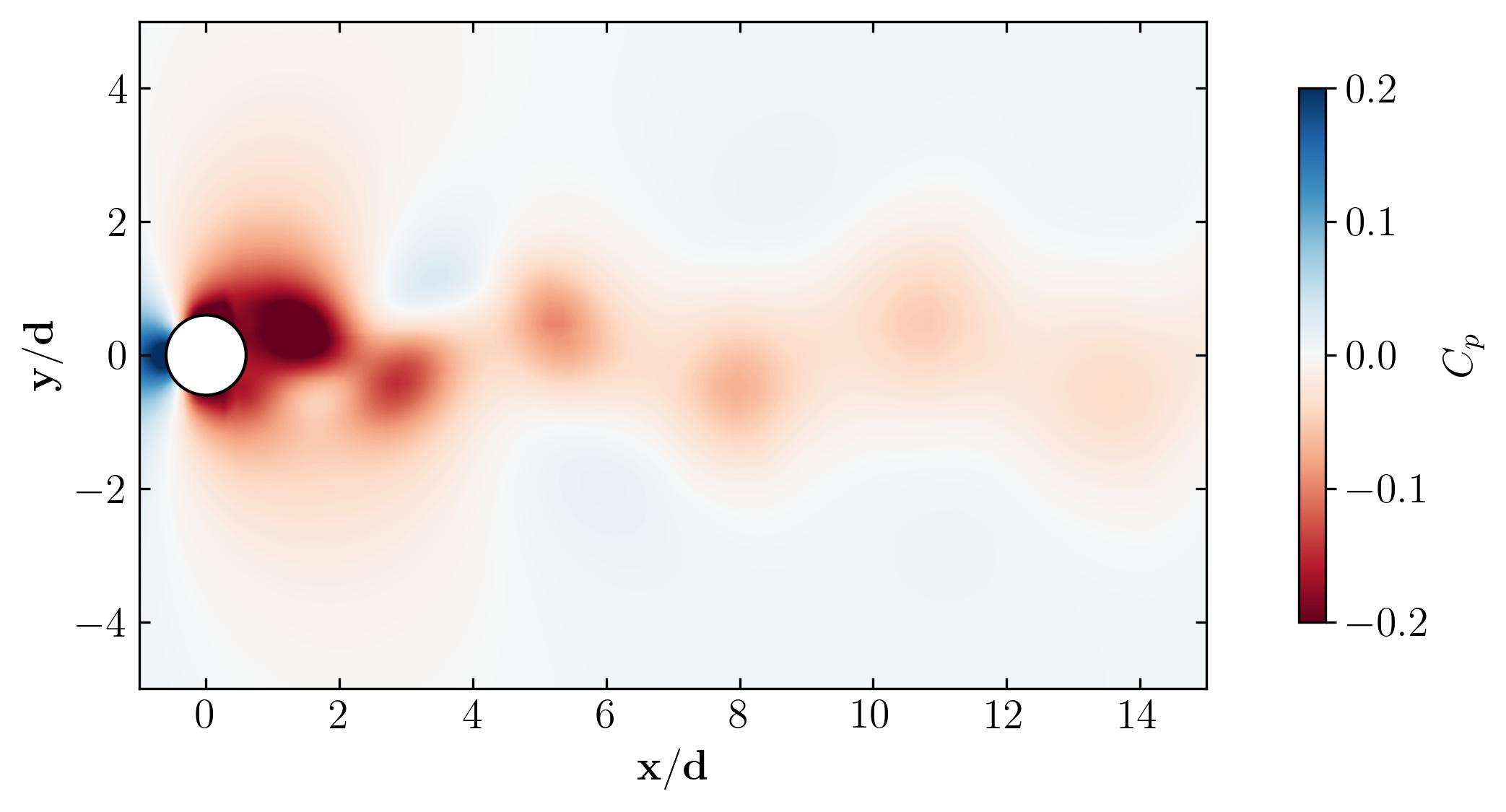
For instance, if high-fidelity results are desired, Direct Numerical Simulation (DNS) offers a viable option. However, this approach demands substantial computational resources due to its ability to resolve all scales of the flow, resulting in close approximation to physical reality. Conversely, Reynolds-Averaged Navier-Stokes (RANS) simulations provide a computationally more economical alternative. Yet, they represent a steady state of inherently unsteady phenomena, potentially limiting their applicability, especially in scenarios involving vortex shedding.

Here are some key considerations:

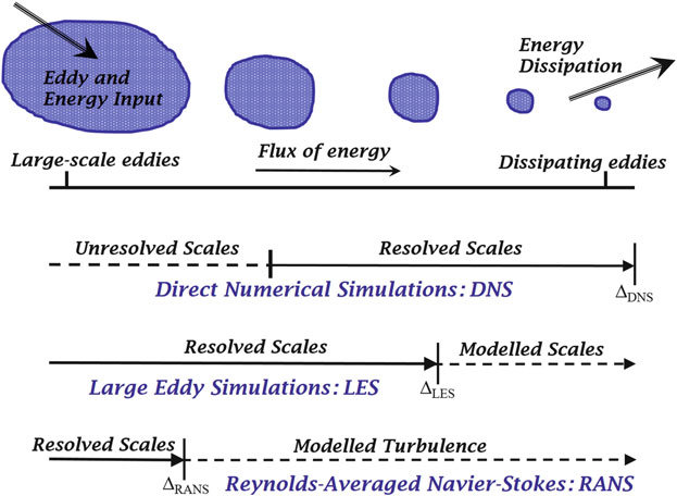
• For numerical investigations at low Reynolds numbers, Direct Numerical Simulations or laminar simulations are preferred. DNS accurately resolves all flow scales, offering precise results.
• At moderate Reynolds numbers, Large Eddy Simulations (LES) strike a balance by resolving large-scale flow structures while modeling near-wall or sub-grid scale features.
• For very large Reynolds numbers, RANS simulations are recommended due to computational constraints. These simulations offer an efficient means of handling turbulent flows.
• In LES, the choice of sub-grid scale models is critical. Options in OpenFOAM include Dynamic k-eqn, Smagorinsky, and others.
• Hybrid RAS-LES approaches like Delayed Detached Eddy Simulation (DDES) and Improved Delayed Detached Eddy Simulation (IDDES) provide additional options for turbulence modeling.
• Various RANS models in OpenFOAM cater to different turbulence modeling needs, ranging from linear to non-linear eddy viscosity and Reynolds stress transport models.

The selection of an appropriate simulation model hinges on factors such as computational grid resolution and resource availability, emphasizing the complexity and depth of methodology involved in CFD simulations.

Gird Independence Analysis

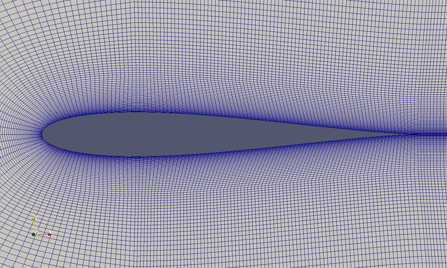
Analyzing grid independence for equations such as 1D convection-diffusion might seem straightforward, but when tackling more complex simulations, like those in 2D or 3D, the task becomes more intricate. Whether dealing with internal or external flow, ensuring grid independence or conducting mesh sensitivity analysis remains crucial. Before delving into the specifics of grid independence, let’s first grasp the concept of the smallest or first cell size. This refers to the size of the initial cell adjacent to any surface, which dictates the expansion of the grid based on the chosen grid aspect ratio.

In scenarios like Direct Numerical Simulations (DNS), the first cell size is determined by Kolmogorov Length Scales, while for methods like Large Eddy Simulations (LES) or Reynolds-Averaged Navier-Stokes (RANS) simulations, it’s estimated using Y-Plus (Y+) or ‘The Law of the Wall’. For DNS, the Kolmogorov microscales can be approximated using a simple Python code,

### Model Parameters

mu = 0.000018375 # dynamic viscosity
rho = 1.225 # density
h = 0.012 # length scale
Re = 1000 # Reynolds number

nu = mu/rho # kinematic viscosity
U_inf = (Re * nu)/h # freestream velocity
epsilon = (U_inf**3)/h # average rate of dissipation of turbulence kinetic energy

### Kolmogorov Length Scale
eta = ((nu**3)/epsilon)**(1/4)

### Kolmogorov Time Scale
tau = (nu/epsilon)**(1/2)

### Kolmogorov Velocity Scale
u_k = (nu*epsilon)**(1/4)

Where eta represents the Kolmogorov length scale, ideally serving as the initial cell spacing for laminar or DNS simulations.

Likewise, the initial cell spacing based on Y-Plus for LES or RANS can be estimated using the online tool provided by Cadence, or through a straightforward Python script, like the following:

### Model Parameters

mu = 0.000018375 # dynamic viscosity
rho = 1.225 # density
h = 0.012 # length scale
Re = 1000 # Reynolds number
U_inf = (Re * nu)/h # freestream velocity

### Yplus Calculation
y_plus = 1 # initial guess
Cf = 0.026/(Re**(1/7))
Tau_Wall = 0.5 * Cf * rho * (U_inf**2)
U_Fric = math.sqrt(Tau_Wall/rho)

Delta_S = (y_plus * nu)/U_Fric ### First cell size

Where Delta_S represents the first cell size based on the estimate of Y-Plus of 1.

Once the first cell size is determined, conducting a grid independence analysis involves employing at least three spatial grids. Personally, I advocate for utilizing four grids with progressively refined meshes. Begin by constructing the finest mesh ideally using the first-cell size estimated by the aforementioned code. Then, refine the grid using a ratio of 2 (or less) to obtain coarser grids. Below is a convenient script for this process:

First_cell_Size = 6.748095902284189e-05 ### Eta value for Re = 1000

Refinement_ratio = 2 ## can be kept between 1.2-2

Grid_1 = First_cell_Size
Grid_2 = Grid_1 * Refinement_ratio
Grid_3 = Grid_2 * Refinement_ratio
Grid_4 = Grid_3 * Refinement_ratio

print('Grid 1 = ', Grid_1)
print('Grid 2 = ', Grid_2)
print('Grid 3 = ', Grid_3)
print('Grid 4 = ', Grid_4)

Following the results from this script, proceed to construct four grids with the specified first cell sizes. Subsequently, conduct your simulations while meticulously monitoring parameters such as the coefficient of drag and lift, mean velocities, turbulent quantities, etc. Afterwards, compile a comprehensive table comparing the coefficients of drag and lift, accompanied by multiple plots showcasing the mean and turbulent quantities for all four grids. For reference, refer to examples from my article in the Journal of Fluid Mechanics.

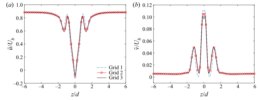
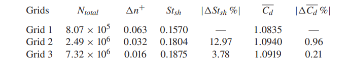
In research, achieving grid independence typically entails ensuring that the percentage difference falls below 5%. However, for scenarios involving complex flow phenomena or turbulent flow simulations, this threshold is often set even lower, below 1%. In essence, a simulation can only be deemed grid independent when the percentage difference in coefficients of drag and lift for two successive refined grids is below 1%.

Time-step Independence Analysis

Fluid dynamics encompasses both spatial and temporal aspects. While grid independence ensures spatial verification, temporal grid verification is achieved through time-step independence analysis. This entails examining how altering the time-step of a transient simulation impacts the results, ensuring that crucial transient effects are adequately resolved and that further reduction in the time-step does not significantly alter results. Integral to this process is understanding the Courant–Friedrichs–Lewy (CFL) condition, a stability criterion for transient simulations. The CFL condition stipulates that the distance any information travels during a time-step within the mesh must be shorter than the distance between mesh elements, ensuring that information propagates only to immediate neighbors without skipping mesh elements.

For more information on how to setup an unsteady OpenFOAM case, follow this link.

To explore the potential impact of time-step adjustments on results, one must verify that such changes do not introduce significant alterations. Consider a scenario where the mesh is established, and the time-step is set based on a CFL value of 0.8 (ideally). For time-step independence analysis, the same simulation must be conducted using the same mesh, but with a reduced time-step. Similar to grid independence, the time-step can be refined by a ratio ranging between 1.2 and 2, indicating a reduction of the time-step by 1.2 or 2 times.

Ideally, time-step independence analysis necessitates only two simulations. The first serves as the base simulation with a CFL value of 0.8, while the second employs a smaller time-step corresponding to a CFL value of 0.4 (if the ratio is 2). Subsequently, the flow results between the two simulations are compared, akin to grid independence analysis.

Check the mass and continuity errors

This step primarily serves as a numerical setup check rather than a verification step. If you’ve ever used OpenFOAM, you’ve likely encountered the following line in the simulation output:

time step continuity errors : sum local = 6.11228e-09, global = 1.51821e-18, cumulative = 1.09644e-17

Here, the “time step continuity errors” refer to the continuity equation error. Essentially, it represents the sum of fluxes over all mesh faces and ideally should equate to zero. Given the nature of numerical simulations, a value like 1.09644e-17 is essentially zero. Throughout your simulations, it’s imperative to ensure that this number doesn’t begin to escalate, as that could lead to divergence in your simulation. Various factors, including initial conditions, solver tolerances, mesh orthogonality, etc., can influence these errors.

Domain independence analysis

An essential aspect of verifying a Computational Fluid Dynamics (CFD) model is ensuring that the boundaries of your computational domain are sufficiently distant—especially if you’re aiming to model a far-field condition—so as not to unduly influence the results. Conducting a sensitivity analysis on the proximity of boundary conditions is crucial, often referred to as Domain Independence. Essentially, this entails testing whether your domain size impacts major flow features, ensuring that the domain size doesn’t introduce significant distortions.

Both internal and external flows can be affected by the placement of outflow boundary conditions, which may lead to numerical instability or pressure reflections (referred to as pressure feedback) that distort the upstream flow. Nearly all boundary conditions come with numerical side effects, often related to pressure blockage. Hence, it’s advisable to position boundary conditions far from the region of interest to mitigate these effects on critical flow regions. However, a larger domain implies a larger grid size and increased computational expense, necessitating an economical estimate of the domain size.

Consider the following example:

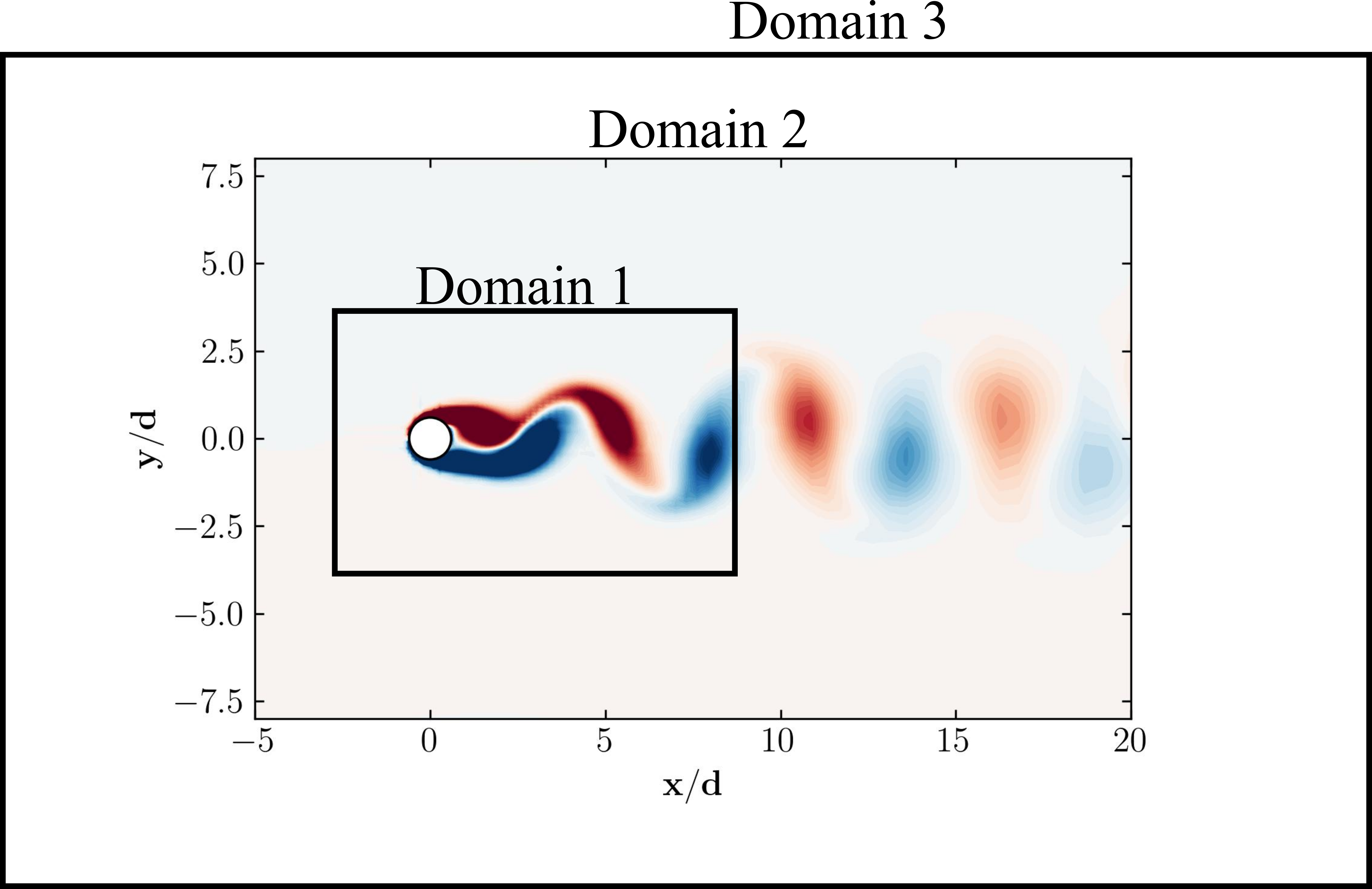
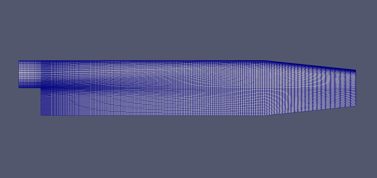
1. Domain 1 is too compact to capture the complete flow physics adequately. Such proximity of the outlet boundary may cause pressure buildup near the cylinder, leading to blockage.
2. Domain 3, conversely, is overly expansive. Despite its size, it would yield results similar to Domain 2 but with a significantly higher computational cost.
3. Domain 2 represents the optimal, verified domain size—economical enough to be computationally feasible yet large enough to yield accurate results.

The ideal domain size varies depending on the specific flow physics, whether internal or external. It’s advisable to consult well-researched studies tailored to your specific case to determine an appropriate domain size. Subsequently, you can conduct domain independence tests by examining domains smaller and larger than the suggested size. This analysis typically confirms that a smaller domain is inadequate, while a larger domain yields results comparable to the optimal “Just Right” domain size.

Validation of numerical setup or flow physics.

When it comes to validation, navigating through the murky waters of academia can be challenging. There’s an unwritten law that states: “Everybody believes an experiment, except the one who did it. And, Nobody believes a simulation result, except the one who did it.” This sentiment resonates with the adage “Garbage in, garbage out,” which applies to CFD as well. The validity of input data, including boundary conditions, setup, and flow conditions, profoundly influences the correctness of the output. Consequently, validation of CFD models becomes an imperative.

As discussed previously, validation occurs through one of two methods: comparing numerical results with experimental data or comparing the numerical setup with known experiments. However, it’s possible that at the parameter space required, no experiments have been conducted. In such cases, validation of the numerical setup—comprising the solver, boundary conditions, and numerical schemes—can be undertaken. Additionally, for validation, numerical results can be compared with another set of numerical results. In this scenario, it’s crucial to compare with a numerical method that is better resolved than yours. For instance, one can compare Reynolds-Averaged Navier-Stokes (RANS) with Large Eddy Simulation (LES) or Direct Numerical Simulation (DNS), but cannot compare RANS with RANS. Similarly, LES can only be compared to DNS, not vice versa. Finally, comparing DNS to DNS is also not advisable.

In summary, it’s essential to remain cognizant of the adage “Garbage in, garbage out,” emphasizing the importance of ensuring the validity of input data. For CFD, don’t forget to verify and validate!!!

Happy computing!!!