Ever wondered what secrets lurk within your CFD simulations? This article delves into the power of Proper Orthogonal Decomposition (POD), a technique for extracting key flow features from OpenFOAM data. We’ll focus on a specific POD method that utilizes Python to analyze field information directly extracted from OpenFOAM time directories. Get ready to unlock hidden patterns and gain deeper insights into your fluid dynamics simulations!

Have you ever stared at the mountains of data generated by your OpenFOAM simulations, wondering what hidden truths they hold? Beneath the surface of velocity vectors and pressure fields lies a symphony of flow features, each playing a crucial role in the grand performance of your fluid dynamics problem. But how do you isolate these key players, separate the signal from the noise, and gain a deeper understanding of the intricate dance within your simulation?

Proper Orthogonal Decomposition (POD) is to the rescue. POD is a powerful mathematical technique that acts as a conductor, drawing out the dominant modes of variation within your data. Imagine being able to decompose the complex flow field into a series of simpler, more interpretable components – like identifying the melody, harmony, and rhythm that combine to form a musical piece. POD achieves just that, allowing you to not only identify the most energetic structures within your simulation, but also quantify their contribution to the overall flow behavior.

This article builds upon my previous two articles (here and here) that delved into the mathematical foundations of POD and provided a concrete example of its application. Here, we’ll take a more practical approach, focusing on a method that leverages the Python programming language to directly analyze field information extracted from OpenFOAM time directories.

We’ll guide you through the implementation of POD within the OpenFOAM CFD workflow, equipping you with the tools to unlock the hidden patterns lurking within your CFD simulations. Get ready to transform your data from a cryptic message into a clear and insightful narrative, empowering you to optimize your models and unlock a new level of understanding in your fluid dynamics research. Lets begin!!

Prerequisites

Setting Up the Case

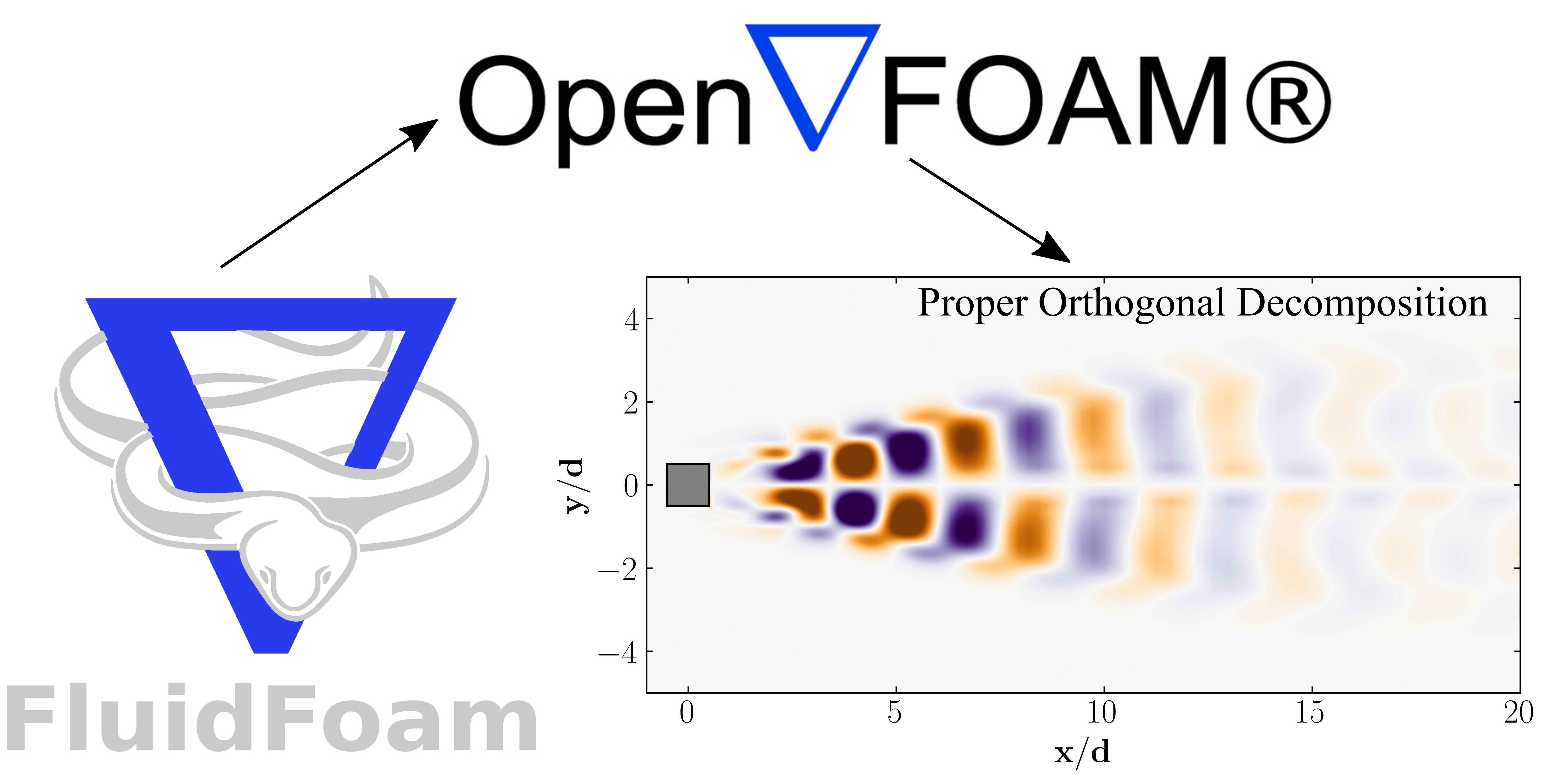
To delve into Proper Orthogonal Decomposition (POD) using a combination of OpenFOAM and Python, our focus will center on examining the dynamics of a two-dimensional flow around a square cylinder at a Reynolds number of 100. This exploration will entail simulating the flow through Direct Numerical Simulations (DNS), employing OpenFOAM as the computational framework. The configuration of this case closely follows the guidelines outlined by Bai and Alam (2018) for reference. You can find detailed instructions in their work.

To ensure alignment with the reference, it’s imperative to follow the prescribed setup meticulously. Refer to this link for a comprehensive guide on prepping your OpenFOAM case for Modal Decomposition.

Verify that your case adheres to the specifications outlined in the reference and includes multiple time directories (snapshots) resembling the format below:

7470.000000116633  7560.000000118597  7650.000000120562  7740.250000122532  7831.250000124518  7922.250000126504
7470.750000116649  7561.750000118635  7651.000000120584  7742.00000012257   7833.000000124556  7924.000000126543
...
7547.75000011833   7638.750000120316  7728.000000122264  7819.000000124251  7910.000000126237  constant
7549.500000118368  7640.500000120354  7729.750000122302  7820.750000124289  7911.750000126275  postProcessing
7551.250000118406  7642.250000120393  7731.500000122341  7822.500000124327  7913.500000126313  system

PRO TIP: Ensure a minimum of 256 snapshots are captured for your data.

Visualization Case Setup

For data visualization purposes, we will establish a separate directory for a second case setup. Begin by duplicating the 0, constant, and system files from your original case into a new directory named visualizationCase. Additionally, within this new directory, create a time directory named 1 to facilitate the organization of your data.

Utilizing FluidFoam

In this article, our exploration heavily leans on a Python package called fluidfoam. This specialized package is crafted specifically for OpenFOAM post-processing tasks. Fluidfoam streamlines intricate operations such as extracting velocity and pressure data from simulations, seamlessly managing OpenFOAM-specific data structures, and facilitating insightful visualizations with minimal complexity.

For instance, extracting the velocity field from within OpenFOAM is simplified using fluidfoam. Here’s an example code snippet:

# import readvector function from fluidfoam package
from fluidfoam import readvector
vel = readvector('Path/To/Your/Case', time_name='latestTime', name='U', structured=False)

In this snippet, vel represents the velocity vector imported into Python from your OpenFOAM case. It reads the latest available time (time_name='latestTime') and any specified fields (name='U'). Other available fields include UMean, UPrime2Mean, p, pMean, etc. The variable vel produces a numpy ndarray of size (3 x NumberOfCells). Transposing the data is necessary to obtain a (NumberOfCells x 3) array:

new_vel = np.reshape(vel.T,(216000,1), order='F')

Here, vel.T denotes the transpose of the velocity vector array, and order='F' ensures the maintenance of element order. 'F' specifies Fortran-like index order, where the first index changes fastest and the last index changes slowest.

After matrix manipulation, the reshaped velocity array can be transformed back to its original format (transpose form) using:

new_vel = np.reshape(new_vel, (72000,3), order='F')

This reshaped matrix retains the same mesh order as the original field and can be effortlessly integrated into OpenFOAM cases for post-processing via tools like Tecplot or ParaView.

Proper Orthogonal Decomposition (POD) with OpenFOAM and Python

Let’s kick off by launching a Jupyter notebook and importing the essential modules:

import matplotlib.colors
import matplotlib.pyplot as plt
import numpy as np
import pandas as pd
import fluidfoam as fl ### Most Important
import scipy as sp
from matplotlib.colors import ListedColormap
import os
import io

%matplotlib inline

plt.rcParams.update({'font.size' : 18, 'font.family' : 'Times New Roman', "text.usetex": True})

Step 1: Setting Up Paths

Begin by assigning paths to your case directory and the folder where you intend to store your data:

Path = 'E:/Blog_Posts/OpenFOAM_POD/Square_Cylinder_Laminar/'
save_path = 'E:/Blog_Posts/OpenFOAM/ROM_Series/Post23/'

Step 2: Extracting Time Directories as a List

Navigate to your OpenFOAM case within a Linux terminal on WSL or Ubuntu. First, within OpenFOAM, execute the command:

foamListTimes | tee times.txt

This command generates a text file named times.txt, listing all the time directory names.

In Python, convert the text file into a list using the following code:

Times = open(Path + 'times.txt').read().splitlines()
Snapshots = len(Times)
print(Snapshots)
### Output
### 256

This method results in Times being a list of strings. For instance, Times[0] = 'xxxx' (a string that can be directly read into the subsequent line of code). The output, indicating the number of snapshots, should match the number of time directories saved in your case.

Step 3: Reading a Velocity Vector Field

Let’s attempt to read a velocity field from OpenFOAM into Python using fluidfoam.

vel = fl.readvector(Path, time_name='latestTime', name='U', structured=False)
columns, rows = np.shape(vel.T)
print(columns, rows)
### Output
### 95868 3

Successfully, we’ve imported a vector field from the OpenFOAM case into Python. Verify and assign the shape of the vector field to determine the number of rows and columns in your dataset, which will prove useful later.

Note: Here, columns correspond to the total number of data points in the internal mesh, while rows represent the velocity components (u, v, and w).

Step 4: Assembling the Mean-Removed Data Matrix

Let’s construct the mean-removed data matrix using fluidfoam.

B = np.zeros((columns*rows,Snapshots)) # Matrix to store the fluctuating velocity field

# Reading the mean velocity field
Mean_vel1 = fl.readvector(Path, time_name=str(Times[0]), name='UMean', structured=False)

for i in np.arange(0,Snapshots):
    vel1 = fl.readvector(Path, time_name=str(Times[i]), name='U', structured=False)
    new_vel1 = np.reshape(vel1.T,(columns*rows,1), order='F')
    new_Mean_Vel1 = np.reshape(Mean_vel1.T,(columns*rows,1), order='F')
    MC = new_vel1 - new_Mean_Vel1
    B[:,i:i+1] = MC

np.save(save_path + 'B.npy', B) ### Save the numpy file

Since we’ve run the case until it reached statistical stability, we can obtain the mean velocity (UMean) using OpenFOAM function objects and then utilize it here to derive the mean-removed matrix, B.

Step 5: POD Algorithm

Next, we form the correlation matrix and perform Singular Value Decomposition (SVD) on it to obtain the eigenvalues and eigenvectors:

C = np.matmul(B.T, B)/len(Times) # Autocorrelation Matrix
S, U = np.linalg.eig(C) # Eigenvalues and Eigenvectors

Subsequently, we obtain the POD modes and compute their modal energy:

### POD modes
Modes = np.matmul(B,U)

### Mode Energy
res = sum([i**2 for i in S])
Energy = np.zeros((len(S),1))
for i in np.arange(0,len(S)):
    Energy[i] = S[i]**2/res

Finally, compute the POD amplitudes:

### POD Normalized Amplitudes
norms = np.linalg.norm(Modes,ord=None, axis=1)
normal_modes = np.zeros((columns*rows,Snapshots))
for i in np.arange(0,Snapshots):
    normals = np.divide(Modes.T[i], norms)
    normal_modes[:,i] = normals

Amp_test = np.matmul(normal_modes.T, B)

At this stage, the POD of your data should be computed. Now, let’s delve into visualizing it.

Data visualization

To prepare the POD modes for visualization, we need to save them to an OpenFOAM native format file, which can then be read into Tecplot or ParaView. First, let’s create two text files named header.txt and footer.txt. Open any vector field file from your time directories and copy the header and footer sections into these text files. Save them in the Path file location.

The contents of the header.txt file should be as follows:

/*--------------------------------*- C++ -*----------------------------------*\
| =========                 |                                                 |
| \\      /  F ield         | OpenFOAM: The Open Source CFD Toolbox           |
|  \\    /   O peration     | Version:  2312                                  |
|   \\  /    A nd           | Website:  www.openfoam.com                      |
|    \\/     M anipulation  |                                                 |
\*---------------------------------------------------------------------------*/
FoamFile
{
    version     2.0;
    format      ascii;
    arch        "LSB;label=32;scalar=64";
    class       volVectorField;
    location    "7470.750000116649";
    object      U;
}
// * * * * * * * * * * * * * * * * * * * * * * * * * * * * * * * * * * * * * //

dimensions      [0 1 -1 0 0 0 0];

internalField   nonuniform List<vector> 
95868
(

And the contents of the footer.txt file should be as follows:

)
;

boundaryField
{
    INLET
    {
        type            fixedValue;
        value           uniform (0.015 0 0);
    }
    OUTLET
    {
        type            zeroGradient;
    }
    TOP
    {
        type            slip;
    }
    BOTTOM
    {
        type            slip;
    }
    SIDE1
    {
        type            slip;
    }
    SIDE2
    {
        type            slip;
    }
    PRISM
    {
        type            noSlip;
    }
}


// ************************************************************************* //

Now, let’s read the header and footer files into Python:

# For Header
with open(Path + 'header.txt') as f:
    header="".join([f.readline() for i in range(23)])  ### 22 is number of rows

# For Footer
with open(Path + 'footer.txt') as f:
    footer="".join([f.readline() for i in range(39)])

We can now save the POD modes into OpenFOAM-readable files by combining the header and footer files with the calculated POD modes:

saveTime = 'E:/Blog_Posts/OpenFOAM_POD/'

for i in np.arange(0,10):
    Mode = np.reshape(np.real(Modes[:,i]), (columns,rows), order='F')
    np.savetxt(saveTime + 'Mode' + str(i+1), Mode, fmt='(%s %s %s)', header=header, footer=footer, comments='')

Don’t forget to rename the object within each of these files to the respective names for simplicity, as follows:

    object      Mode1;

Finally, after changing the object name, copy these files into the time directory of visualizationCase we created earlier.

Results

To visualize the results, we can employ either ParaView or Tecplot for post-processing. However, another method involves utilizing the OpenFOAM vtk file extractions. While the first method is straightforward, let’s explore the second one instead.

Begin by utilizing the surfaces function object executed through the command-line. Set up a surfaces file within the system directory as shown below:

/*--------------------------------*- C++ -*----------------------------------*\
  =========                 |
  \\      /  F ield         | OpenFOAM: The Open Source CFD Toolbox
   \\    /   O peration     |
    \\  /    A nd           | Web:      www.OpenFOAM.com
     \\/     M anipulation  |
-------------------------------------------------------------------------------
Description
    Writes out values of fields from cells nearest to specified locations.

\*---------------------------------------------------------------------------*/
surfaces
{
    type            surfaces;
    libs            ("libsampling.so");
    writeControl   	timeStep;
    writeInterval   10;

    surfaceFormat   vtk;
	
	formatOptions
	{
		vtk
		{
			legacy true;
			format ascii;
		} 
	}
	
    fields          (p U Mode1 Mode2 Mode3 Mode4 Mode5 Mode6 Mode7 Mode8 Mode9 Mode10);

    interpolationScheme cellPoint;

    surfaces
    {
        zNormal
        {
            type        cuttingPlane;
            point       (0 0 0);
            normal      (0 0 1);
            interpolate true;
        }
    };
};
// ************************************************************************* //

Now, let’s proceed to extract the data using the postProcess utility with the command:

postProcess -func surfaces

Executing this command will generate a file named surfaces within the postProcessing directory, containing the surface field in a vtk file, as shown below:

surfaces/
└── 1
    └── zNormal.vtp

This vtk file can be readily opened in ParaView or VisIt for visualization. However, today we will visualize these fields in Python using the PyVista module. PyVista is a powerful tool for 3D data visualization, serving as an interface for the Visualization Toolkit (VTK). With PyVista, one can easily read and extract data from a vtk file. In your Jupyter file, start by importing the module:

import pyvista as pv

Then set the path variables:

PathToSurfaces = 'E:/Blog_Posts/OpenFOAM_POD/TestCase/postProcessing/surfaces/1/'
Files = os.listdir(PathToSurfaces)

Now, extract the VTK file using the PyVista module:

Data = pv.read(PathToSurfaces + Files[0])
grid = Data.points
x = grid[:,0]
y = grid[:,1]
z = grid[:,2]
rows, columns = np.shape(grid)
print('rows = ', rows, 'columns = ', columns)

Check which arrays are available within this extracted vtk file:

print(Data.array_names)

Output:

['TimeValue', 'p', 'Mode1', 'Mode10', 'Mode2', 'Mode3', 'Mode4', 'Mode5', 'Mode6', 'Mode7', 'Mode8', 'Mode9', 'U']

Extract the POD modes from the Data:

Mode1 = Data['Mode1']
Mode2 = Data['Mode2']
Mode3 = Data['Mode3']
Mode4 = Data['Mode4']
Mode5 = Data['Mode5']
Mode6 = Data['Mode6']
Mode7 = Data['Mode7']
Mode8 = Data['Mode8']
Mode9 = Data['Mode9']
Mode10 = Data['Mode10']

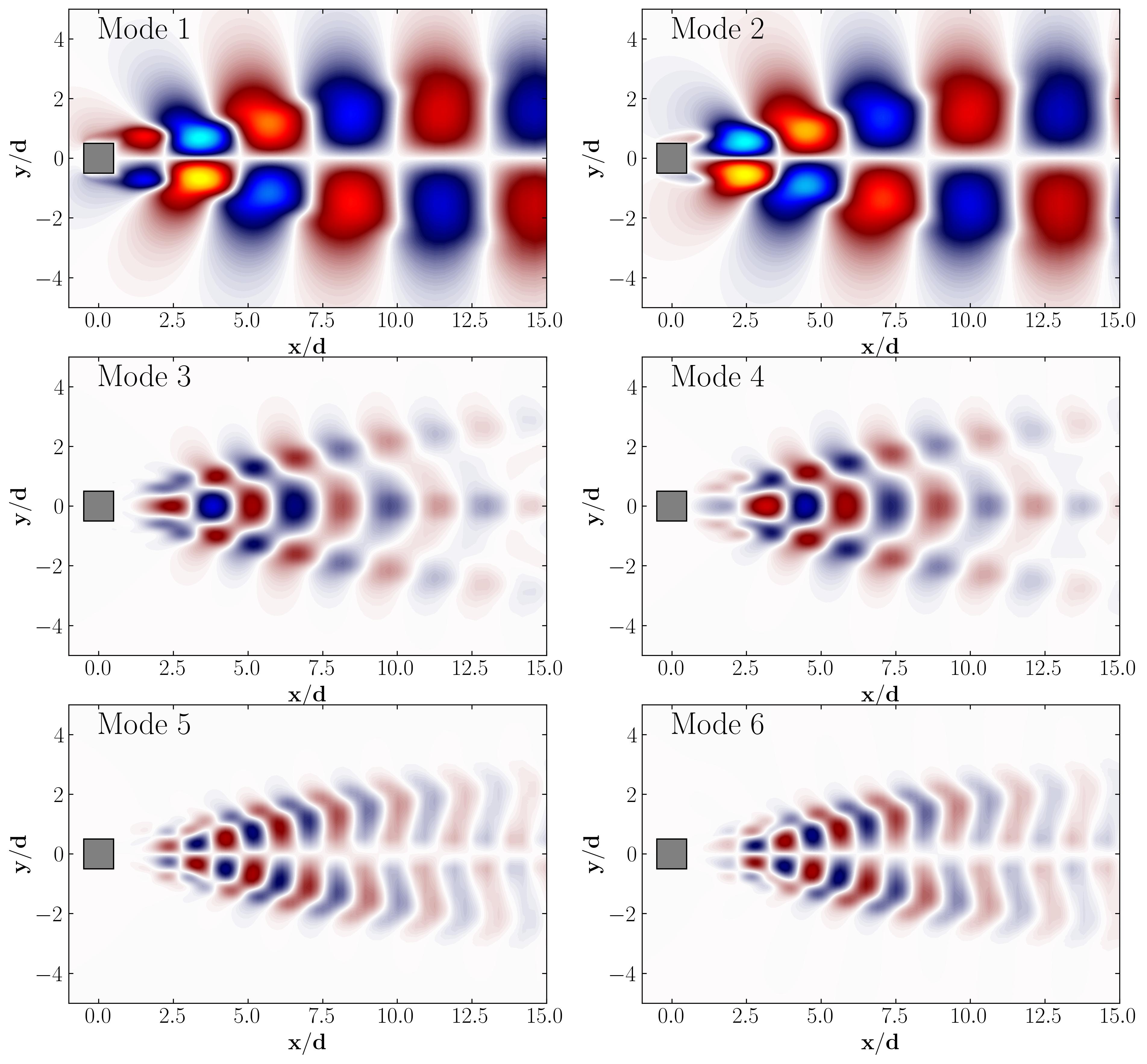
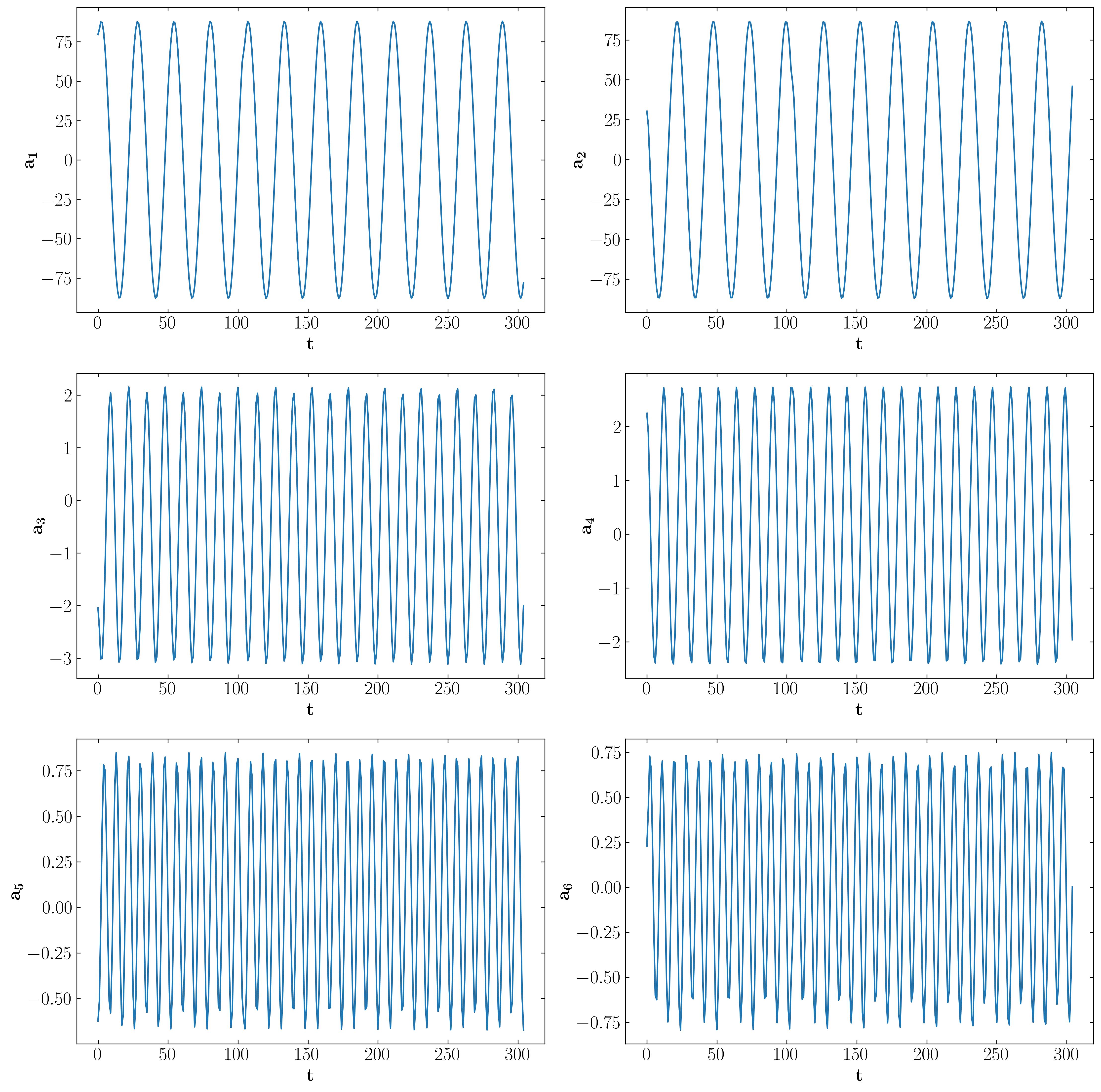
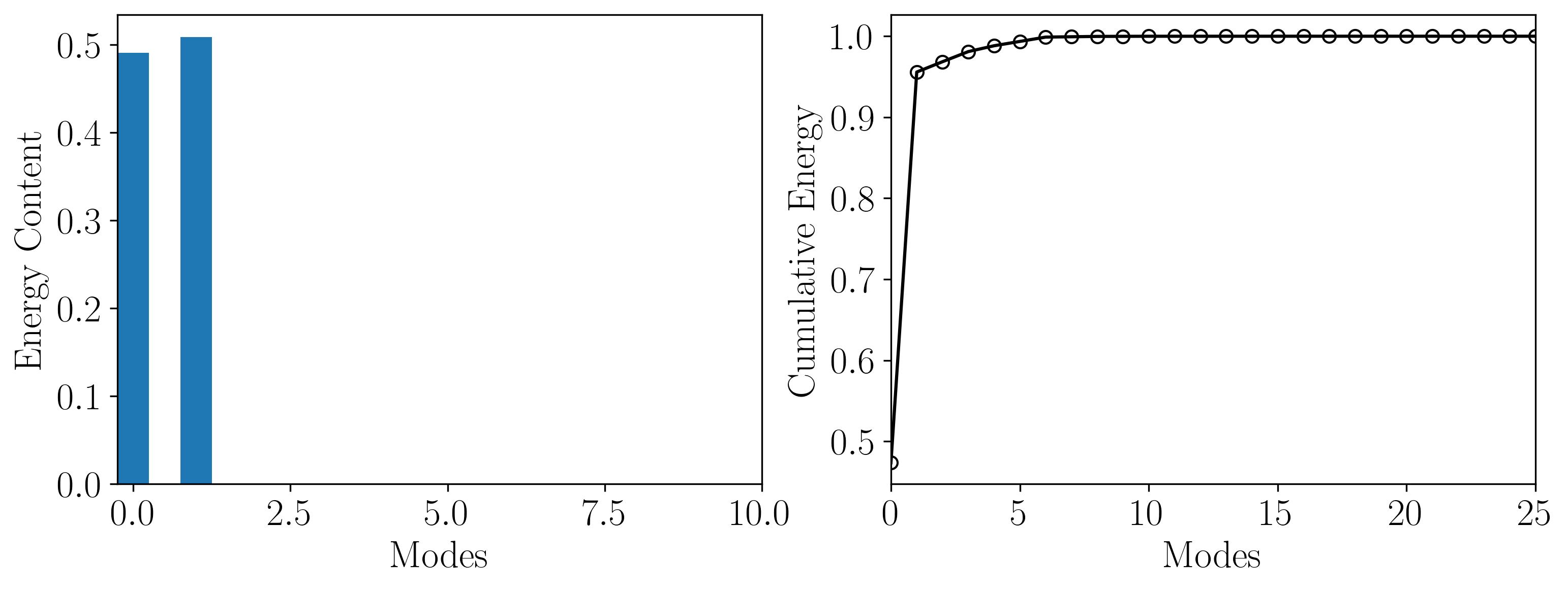
Then simply plot the POD modes, their respective amplitudes, and modal energy using normal matplotlib routines. The results should show up as follows:

POD Modes

Mode Amplitudes

Modal Energy

In conclusion, Proper Orthogonal Decomposition (POD) presents a powerful technique for extracting dominant flow structures and reducing computational complexity in fluid dynamics simulations. Through this article, we’ve navigated the process of setting up a POD analysis using OpenFOAM and Python, from preprocessing to visualization.

In our next article, we’ll delve deeper into the application of POD utilizing surface extraction data from OpenFOAM. Stay tuned as we explore advanced techniques for extracting valuable insights from fluid flow simulations.

Until then, happy coding and happy simulating!