This article empowers you to harness the capabilities of Python scripting for performing POD analysis on 2D slice data extracted from your OpenFOAM simulations. We’ll guide you through the process of leveraging Python’s libraries to unlock hidden patterns within your data, transforming your 2D slices from raw information to a deeper understanding of the key flow dynamics at play.

Imagine peering into a swirling vortex within your OpenFOAM simulation. The complex dance of velocity vectors and pressure fields might seem like a chaotic blur. But beneath the surface lies a hidden order, a symphony of flow features playing a crucial role in the overall performance. Proper Orthogonal Decomposition (POD) acts like a maestro, wielding the power of mathematics to isolate and analyze these dominant modes within your data.

This article delves into the world of POD analysis, specifically focusing on its application to 2D slice data extracted from your OpenFOAM simulations. In this you will discover how to leverage Python’s powerful libraries to directly analyze your 2D slice data, performing POD calculations and visualizing the extracted modes. By the end of this journey, you’ll be equipped to transform your understanding of OpenFOAM data. We’ll go beyond the raw numbers, empowering you to extract hidden patterns, identify key flow features, and gain a richer perspective on the dynamics at play within your simulations. This newfound knowledge can be instrumental in optimizing your models, validating results, and ultimately, unlocking deeper insights into your fluid dynamics research.

Lets begin!!!

Setting Up the Case

In this article, we delve into the intricacies of setting up Proper Orthogonal Decomposition (POD) using OpenFOAM slices and Python. Our focus lies on analyzing the two-dimensional flow around a square cylinder at a Reynolds number of 100. This configuration closely adheres to the guidelines laid out by Bai and Alam (2018) for reference, ensuring a robust methodology. Detailed instructions for this setup are available in their work, providing invaluable guidance for alignment. A comprehensive guide to prepping your OpenFOAM case for Modal Decompositions is available below, offering detailed insights into the necessary steps.

Link to A Guide to Prepping Your OpenFOAM Case for Modal Decompositions.

Our journey begins with a fully-developed, statistically steady flow around a square cylinder at a Reynolds number of 100, as discussed in our previous article. Here, we extend our analysis by running this case for an additional 100 vortex shedding cycles. Within each shedding cycle, we extract two-dimensional slices or surfaces from the data 16 times. The extraction of 2D slices is facilitated by utilizing the surfaces function object in OpenFOAM, as illustrated below:

surfaces
{
    type            surfaces;
    libs            ("libsampling.so");
    writeControl   	timeStep;
    writeInterval   142;

    surfaceFormat   vtk;
    fields          (p U);

    interpolationScheme cellPoint;

    surfaces
    {
        zNormal
        {
            type        cuttingPlane;
            point       (0 0 0.05);
            normal      (0 0 1);
            interpolate true;
        }
    };
};
// ************************************************************************* //

Once the simulation run is complete, you should find a directory named surfaces within the postProcessing directory of your case, containing all the extracted surfaces.

surfaces/
├── 4771.2000000577236
│   └── zNormal.vtp
├── 4772.6200000577546
│   └── zNormal.vtp
├── 4774.0400000577856
│   └── zNormal.vtp
├── 4775.4600000578166
│   └── zNormal.vtp
.
.
.

Ensure that both the case and the surfaces are extracted before proceeding further.

Extracting data from surfaces

To extract data from the VTK files obtained from the OpenFOAM case, we will utilize PyVista. PyVista serves as a helper module for the Visualization Toolkit (VTK), wrapping the VTK library through NumPy and allowing direct array access via various methods and classes. This package offers a Pythonic, well-documented interface that exposes VTK’s robust visualization backend, facilitating rapid prototyping, analysis, and visual integration of spatially referenced datasets.

PyVista proves invaluable for scientific plotting in presentations and research papers, serving also as a supporting module for other Python modules dependent on mesh 3D rendering. Refer to Connections for a list of projects leveraging PyVista.

Let’s initiate a Jupyter notebook and import the necessary modules, including PyVista:

import matplotlib.colors
import matplotlib.pyplot as plt
import numpy as np
import pandas as pd
import fluidfoam as fl
import scipy as sp
import os
import pyvista as pv
import imageio
import io

%matplotlib inline
plt.rcParams.update({'font.size' : 18, 'font.family' : 'Times New Roman', "text.usetex": True})

Setting Path Variables and Constants:

### Constants
d = 0.1
Ub = 0.015

### Paths
Path = 'E:/Blog_Posts/Simulations/Sq_Cyl_Surfaces/surfaces/'
save_path = 'E:/Blog_Posts/SquareCylinderData/'

Files = os.listdir(Path)

Now, let’s attempt to read the first snapshot surface using PyVista:

Data = pv.read(Path + Files[0] + '/zNormal.vtp')
grid = Data.points
x = grid[:,0]
y = grid[:,1]
z = grid[:,2]
rows, columns = np.shape(grid)
print('rows = ', rows, 'columns = ', columns)

print(Data.array_names)

Output:

['TimeValue', 'p', 'U']

Here, we observe that our 2D slices encompass velocity and pressure fields. Leveraging PyVista, we can extract the vorticity field for each snapshot and organize the resulting data into a large, tall, and slender matrix to facilitate POD computation.

Data = pv.read(Path + Files[0] + '/zNormal.vtp')
grid = Data.points
x = grid[:,0]
y = grid[:,1]
z = grid[:,2]
rows, columns = np.shape(grid)
print('rows = ', rows, 'columns = ', columns)

### For U
Snaps = len(Files) # Number of snapshots
data_Vort = np.zeros((rows,Snaps-1))
for i in np.arange(0,Snaps-1):
    data = pv.read(Path + Files[i] + '/zNormal.vtp')
    gradData = data.compute_derivative('U', vorticity=True)
    grad_pyvis = gradData.point_data['vorticity']
    data_Vort[:,i:i+1] = np.reshape(grad_pyvis[:,2], (rows,1), order='F')

np.save(save_path + 'VortZ.npy', data_Vort)

Let’s examine the size of the matrix we’re dealing with by querying the shape of the data_Vort array:

data_Vort.shape
### OUTPUT
### (96624, 1600)

Additionally, we can visualize a snapshot of the vorticity field:

Moreover, for a more dynamic representation (showing off, in other words), we can animate the vorticity field:

Proper Orthogonal Decomposition using 2D slice Data

At this stage, it becomes evident that we will embark on the Proper Orthogonal Decomposition (POD) of the extracted vorticity field data. Below are the steps for implementing the POD algorithm:

### Obtain the Mean-Removed Vorticity
Vort_mean = np.mean(data_Vort, axis=1)
VortPrime = np.zeros((data_Vort.shape[0], data_Vort.shape[1]))
for i in np.arange(0, data_Vort.shape[1]):
    VortPrime[:, i] = data_Vort[:,i] - Vort_mean

### Obtain the Covariance Matrix
uC = np.matmul(VortPrime.T, VortPrime)/data_Vort.shape[1]

### Obtain the Eigenvalues and Eigenvectors
uEVal, uEVec = np.linalg.eig(uC)
uModes = np.matmul(VortPrime,uEVec)

Results

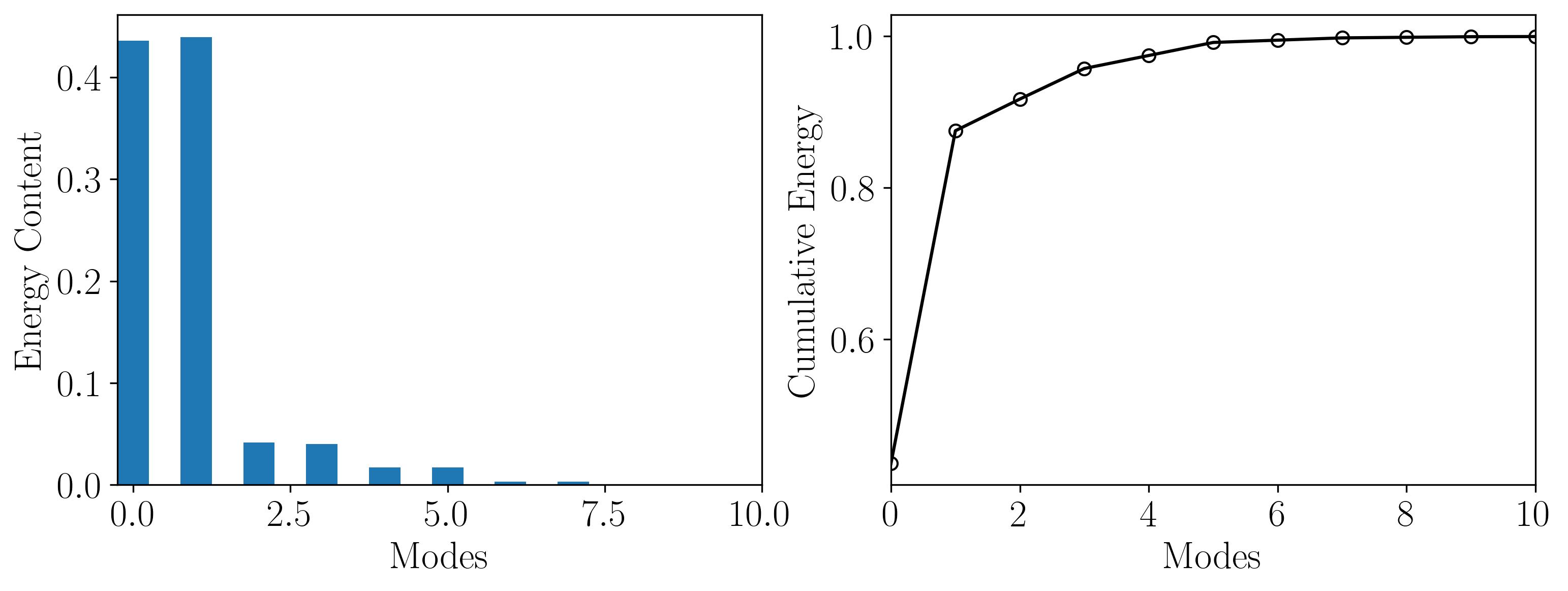
POD Modes

POD Modal Energy

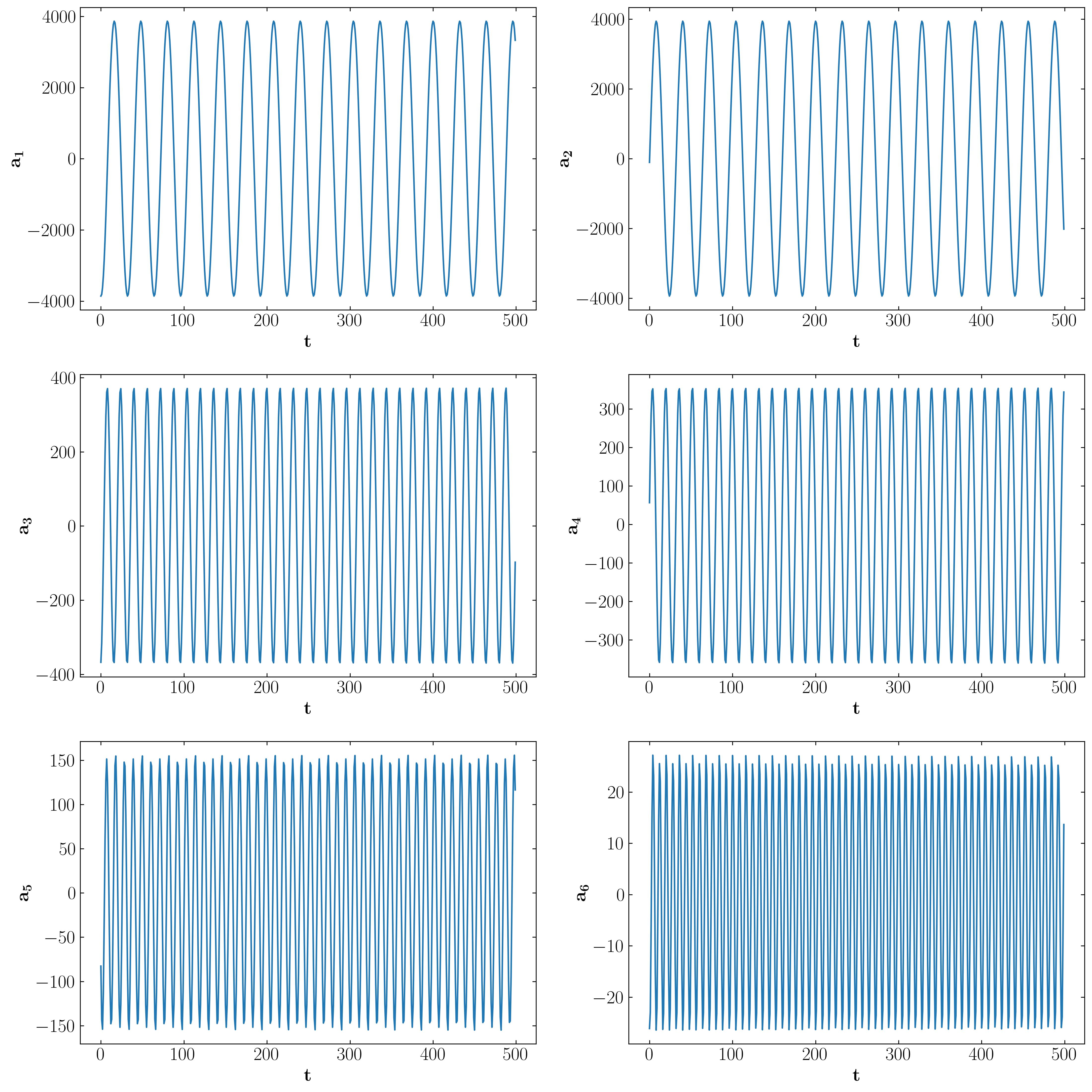
POD Mode Amplitudes

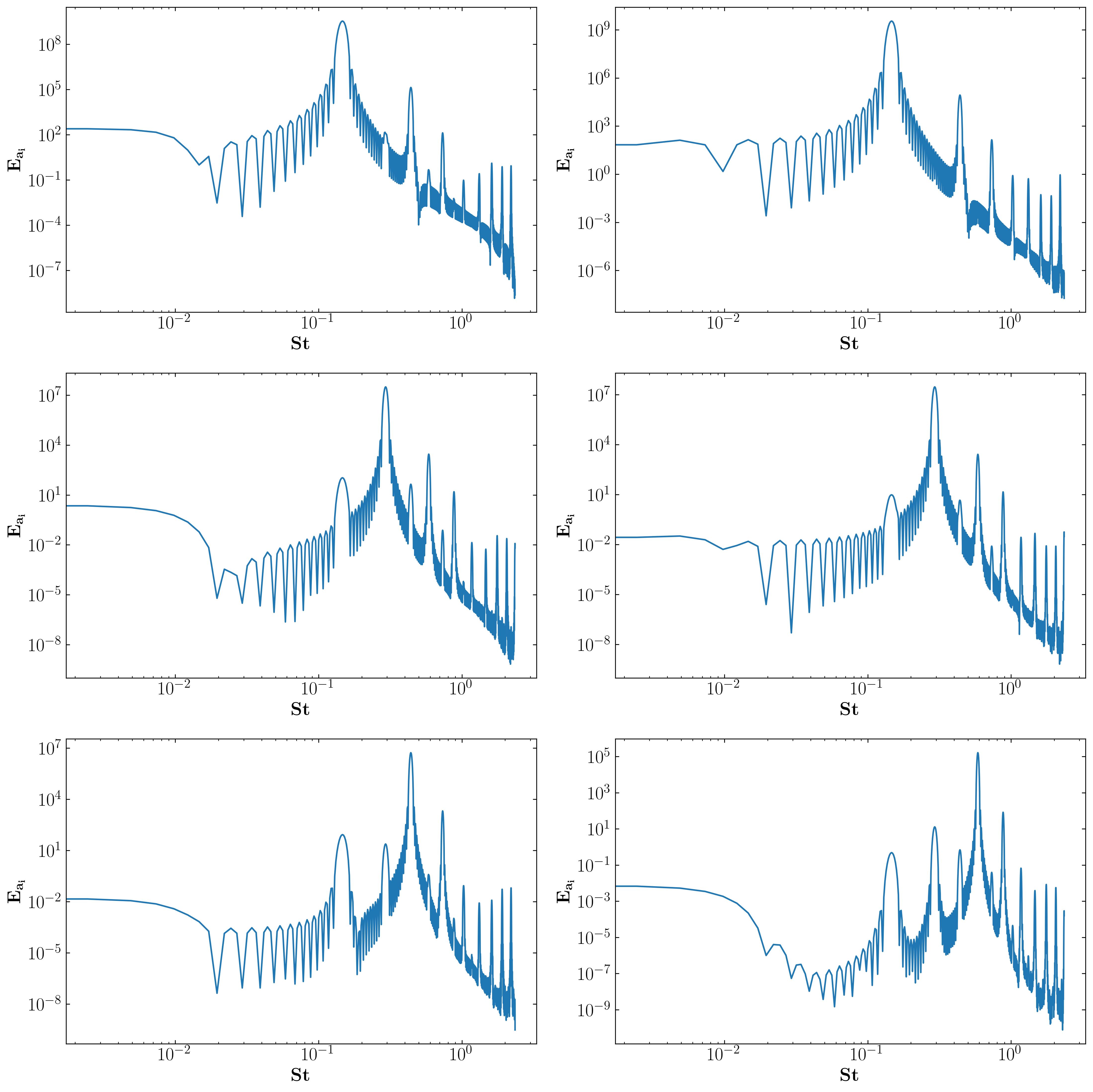
Mode Amplitude FFT

With this, I conclude my series on Proper Orthogonal Decomposition (POD). We explored the mathematical underpinnings, implementation techniques, and diverse applications of POD in fluid mechanics. This series showcased POD’s versatility as a data-driven analysis tool, highlighting its potential to revolutionize flow control, turbulence modeling, and other areas. As research in POD and similar techniques continues alongside advancements in computational tools, we can unlock new avenues for understanding and manipulating complex flow phenomena, ultimately leading to breakthroughs in various scientific and engineering fields.

Moving forward, POD holds immense promise for unlocking new avenues in understanding and manipulating complex flow phenomena. Continued advancements in computational fluid dynamics and data analysis methodologies will see Modal Decomposition method such as POD play a crucial role in areas like optimizing wind turbine performance or even developing novel microfluidic devices. The potential for innovation and discovery in the realm of fluid dynamics remains vast and exciting.