Building upon our exploration of Dynamic Mode Decomposition (DMD), this article takes a practical turn! We’ll leverage a toy example to unveil how DMD tackles the challenge of understanding and predicting complex, nonlinear systems.

In our ongoing exploration of understanding data-driven dynamical systems through modal decomposition methods, our focus has centered on Dynamic Mode Decomposition (DMD). Previously, I introduced the fundamental concepts of DMD and elucidated the mathematical underpinnings in detail. For those seeking a broader introduction to DMD, you can find it in my previous article linked here.

Additionally, for a deeper dive into the mathematical preliminaries of DMD, refer to this article.

In this installment, we’ll delve into the practical application of the DMD algorithm using a toy example. Our objective is to gain insights into diagnosing and predicting nonlinear dynamical systems. Throughout this article, I’ll draw upon insights from the book “Dynamic Mode Decomposition: Data-Driven Modeling of Complex Systems” by J. Nathan Kutz and others.

Let’s dive in!

Recap

Dynamic Mode Decomposition (DMD) offers a powerful method for unraveling complex spatio-temporal dynamics from data, breaking it down into dynamic modes derived from snapshots or measurements over time. This technique shares mathematical principles with the Arnoldi algorithm, a cornerstone of fast computational solvers. The data collection process hinges on two key parameters: 𝑛, representing spatial degrees of freedom per snapshot, and 𝑚, denoting the number of snapshots.

The definition of DMD, as elucidated by Tu et al. (2014), is as follows:

Consider a dynamical system and two sets of data:

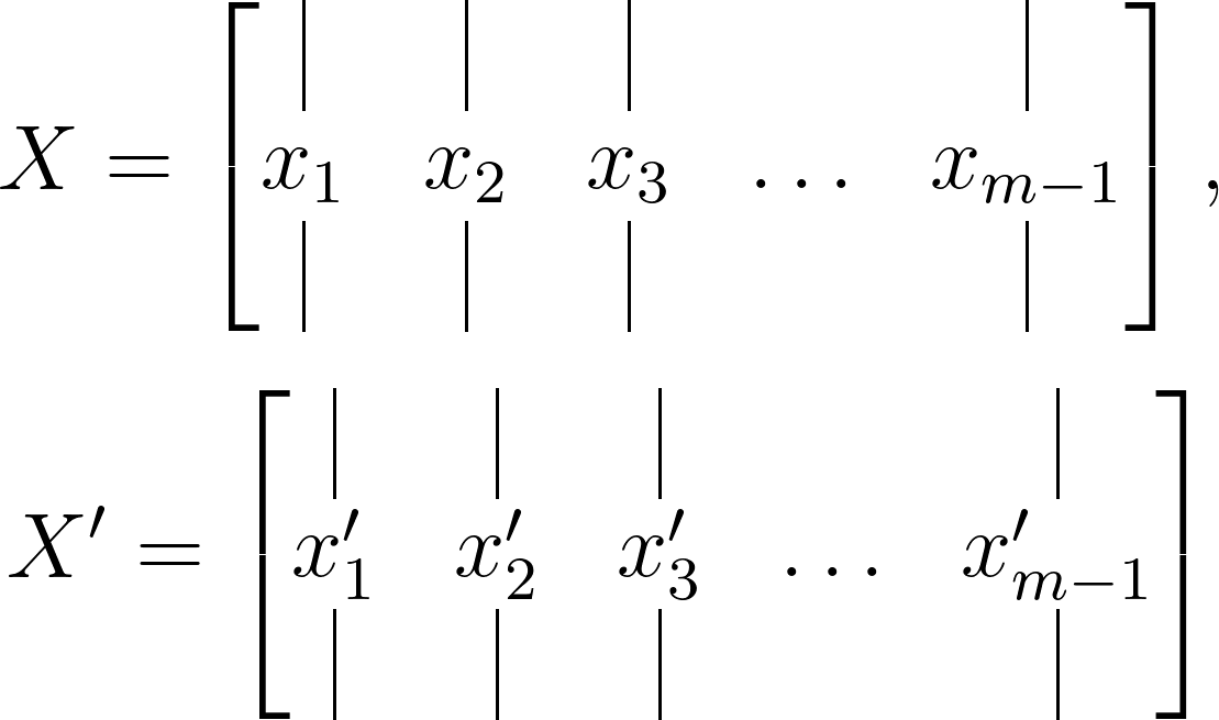
where the temporal evolution of the system over a time interval Δ𝑡 is expressed by a mapping given as:

DMD undertakes the leading eigendecomposition of the best-fit linear mapping operator 𝐴 relating the data matrices:

such that:

The resulting DMD modes, also known as dynamic modes, are the eigenvectors of 𝐴, with each mode corresponding to a specific eigenvalue.

The Algorithm

In practical applications, the state dimension (𝑛) tends to be significantly larger than the number of snapshots (𝑚). Consider, for instance, a numerical fluid dynamics simulation, where 𝑛 represents the number of spatial degrees of freedom and 𝑚 denotes the number of snapshots, each taken Δ𝑡 time apart. In such cases, 𝑛≫𝑚, rendering the matrix 𝐴 dauntingly complex to analyze. Building upon our previous discussions, the DMD methodology sidesteps the eigendecomposition of 𝐴 by adopting a low-rank, reduced-order representation of 𝐴 in terms of the Proper Orthogonal Decomposition-projected matrix $\tilde{A}$.

Below is a step-by-step outline of the Dynamic Mode Decomposition algorithm.

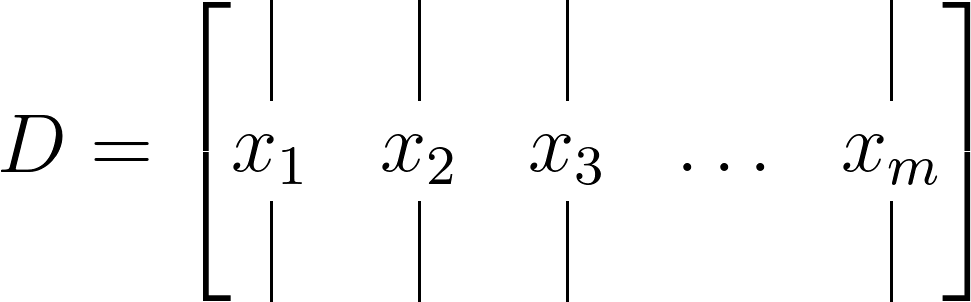
Step 1 : Construct the Data Matrix

Commence by constructing a data matrix as depicted below:

Subsequently, divide this data matrix into two matrices, each time-shifted by Δ𝑡, as illustrated below:

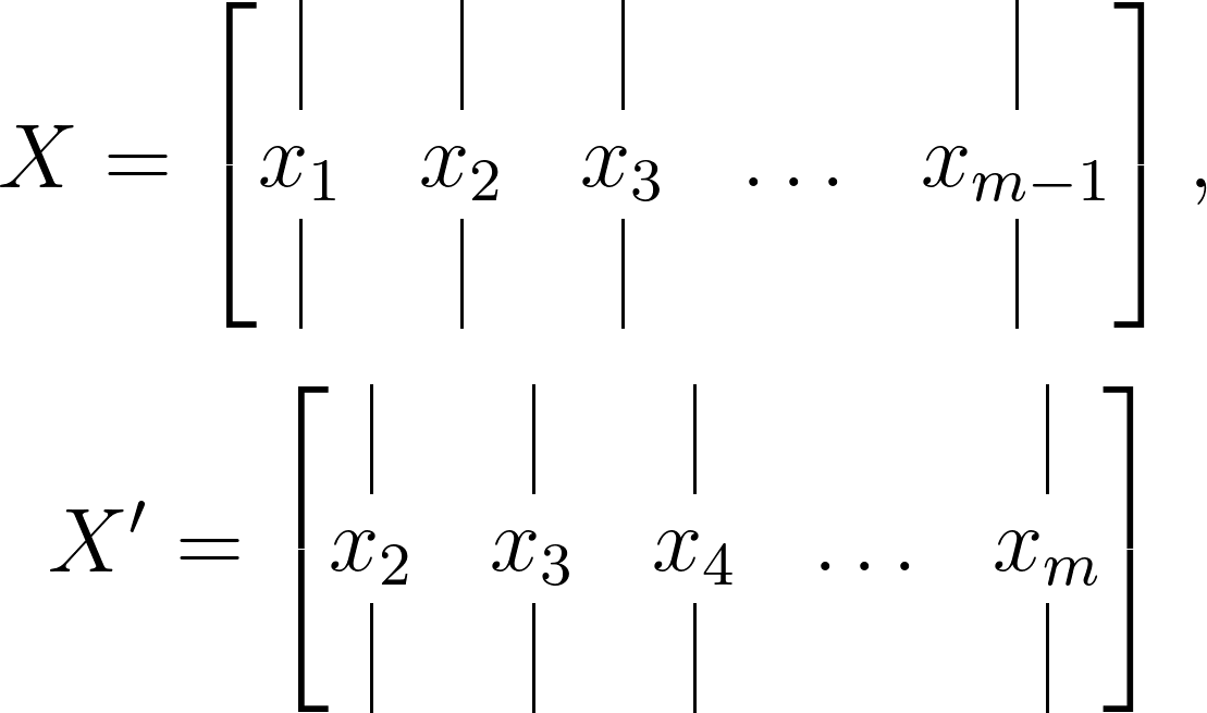
The dimensions of the data matrix will be 𝑛×𝑚, while the time-shifted matrices will measure 𝑛×(𝑚−1).

Step 2 : SVD of X

Initiate by performing the Singular Value Decomposition (SVD) of your first data matrix 𝑋, yielding:

where ∗ denotes the conjugate transpose. The dimensions of 𝑈 will be 𝑛×𝑟, Σ will be 𝑟×𝑟, and 𝑉 will be 𝑚×𝑟. Here, 𝑟 represents the rank of the reduced SVD approximation of 𝑋, and the left singular vectors 𝑈 correspond to the Proper Orthogonal Decomposition (POD) modes of 𝑋.

This stage of the algorithm leverages the SVD to execute a low-rank truncation of the data. Notably, if the data exhibits low-dimensional structure, the singular values of Σ will sharply diminish, potentially leaving only a limited number of dominant modes.

Step 3 : Obtain Matrix A

Recalling the relationship:

Using the SVD approximation from the previous step, we can derive the matrix 𝐴 using the pseudo-inverse of 𝑋 as follows:

However, in practice, it’s more efficient to compute the $\tilde{A}$ matrix, which, after the SVD reduction, represents the 𝑟×𝑟 projection of the full matrix 𝐴 onto the Proper Orthogonal Decomposition (POD) modes:

Here, the matrix $\tilde{A}$ signifies a low-dimensional linear model of the dynamical system on POD coordinates, given as:

It’s also possible to construct the high-dimensional state 𝑥𝑘 as follows:

Step 4 : Compute eigendecomposition

Performing the eigendecomposition of the $\tilde{A}$ matrix results in:

where 𝑊 represents the eigenvectors and 𝛬 is a diagonal matrix containing the corresponding eigenvalues 𝜆𝑘.

Step 5 : Obtain DMD Modes

Finally, we can reconstruct the eigendecomposition of 𝐴 using 𝑊 and 𝛬. Since the $\tilde{A}$ matrix is a reduced representation of 𝐴, the eigenvalues of 𝐴 are given by 𝛬, and the eigenvectors of 𝐴 are obtained from the columns of Φ:

Here, the modes given by Φ are the exact DMD modes. Another set of modes, known as projected DMD modes, are given by:

To find a dynamic mode of 𝐴 associated with a zero eigenvalue 𝜆𝑘=0, the exact DMD mode formulation may be used if Φ is non-zero. Otherwise, the projected DMD mode should be used. In any case, the exact DMD modes represent the dynamic modes we have been seeking!

Prediction

With the low-rank approximations of both the eigenvalues and eigenvectors from the above steps, it becomes possible to predict the future state of the system. This process begins by obtaining 𝜔𝑘 such that:

Then, the approximate solution for all future times is given by:

Here, $𝑏_𝑘$ represents the initial amplitude of each mode, Φ is the matrix whose columns are the DMD eigenvectors $\Phi_𝑘$, and 𝛺=diag(𝜔) is a diagonal matrix whose entries are the eigenvalues $\omega_k$. The eigenvectors $\phi_k$ are the same size as the state 𝑥, and 𝑏 is a vector of the coefficients $b_k$.

In simpler terms, the above equation can be interpreted as a least-squares fit or regression of a best-fit linear dynamical system based on the sampled data:

The matrix 𝐴 is reconstructed by minimizing the least-squares 𝐿2 norm:

Finally, the initial coefficient matrix is computed considering the initial snapshot 𝑥1 at time $t_1=0$, equating $x_1 = \phi b$. Since the matrix of eigenvectors Φ is generally not a square matrix, the initial conditions can be formulated by taking the pseudo-inverse of Φ:

Python implementation

Below is a Python implementation of the DMD algorithm. This function utilizes the low dimensionality inherent in the data to create a low-rank approximation of the linear mapping, which effectively approximates the nonlinear dynamics observed in the system.

def DMD(X1, X2, r, dt):
    U, s, Vh = np.linalg.svd(X1, full_matrices=False)
    ### Truncate the SVD matrices
    Ur = U[:, :r]
    Sr = np.diag(s[:r])
    Vr = Vh.conj().T[:, :r]
    
    ### Build the Atilde and find the eigenvalues and eigenvectors
    Atilde = Ur.conj().T @ X2 @ Vr @ np.linalg.inv(Sr)
    Lambda, W = np.linalg.eig(Atilde)
    
    ### Compute the DMD modes
    Phi = X2 @ Vr @ np.linalg.inv(Sr) @ W
    
    omega = np.log(Lambda)/dt ### continuous time eigenvalues
    
    ### Compute the amplitudes
    
    alpha1 = np.linalg.lstsq(Phi, X1[:, 0], rcond=None)[0] ### DMD mode amplitudes
    
    b = np.linalg.lstsq(Phi, X2[:, 0], rcond=None)[0] ### DMD mode amplitudes
    
    ### DMD reconstruction
    time_dynamics = None
    for i in range(X1.shape[1]):
        v = np.array(alpha1)[:,0]*np.exp( np.array(omega)*(i+1)*dt)
        if time_dynamics is None:
            time_dynamics = v
        else:
            time_dynamics = np.vstack((time_dynamics, v))
    X_dmd = np.dot( np.array(Phi), time_dynamics.T)
    
    return Phi, omega, Lambda, alpha1, b, X_dmd

Toy Example

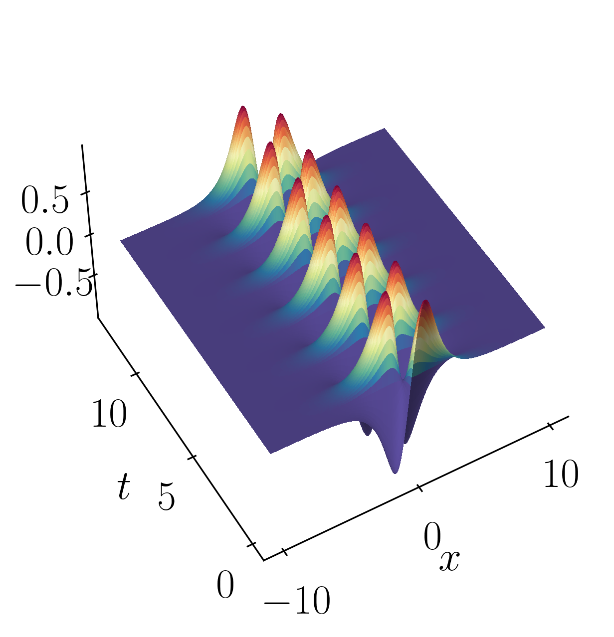
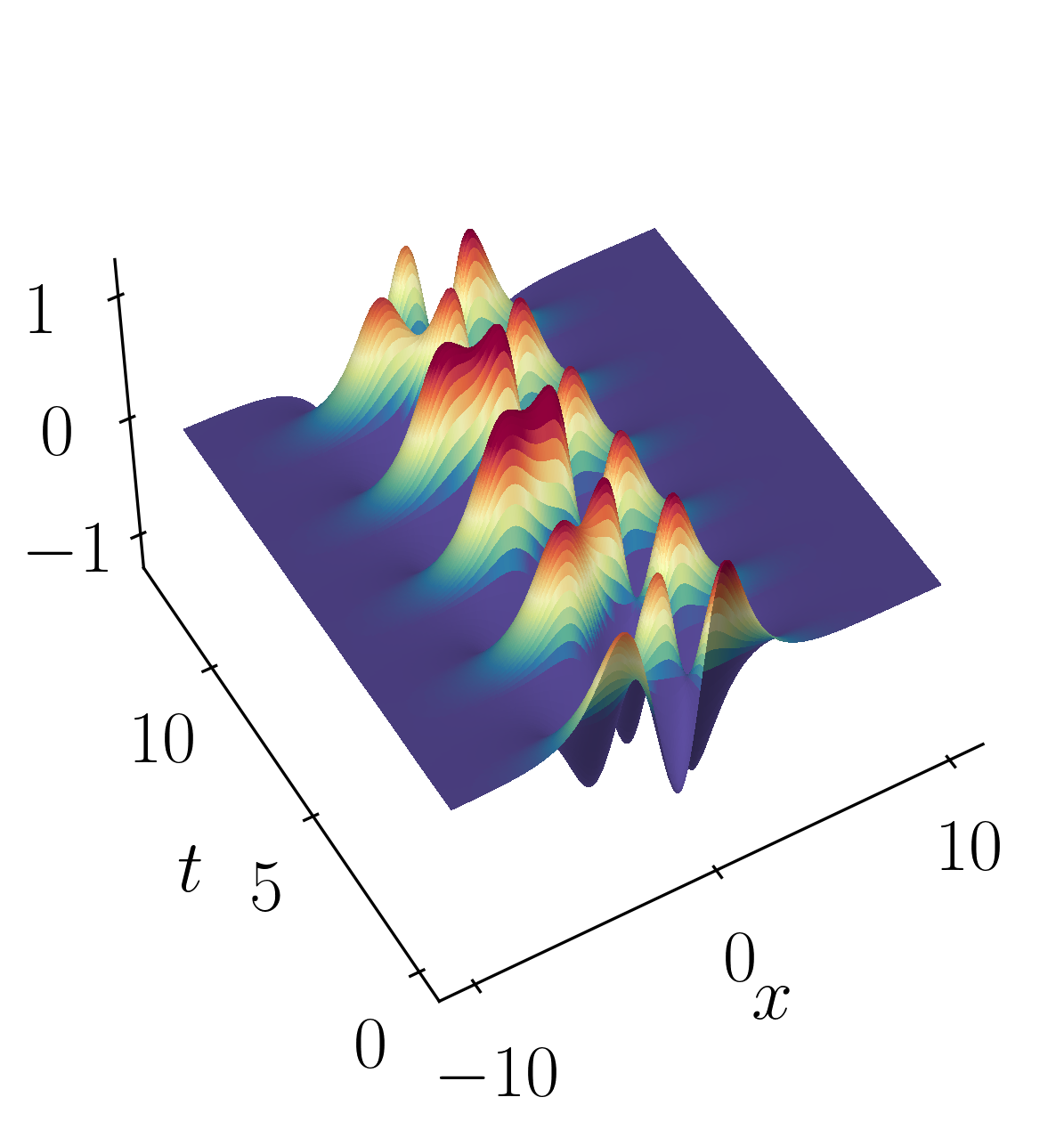
Let’s look into a toy example to illustrate the inner workings of the DMD algorithm outlined above. We’ll examine a simple scenario involving two mixed spatio-temporal signals, akin to the animation at the beginning of this article. The goal here is to showcase how DMD efficiently decomposes the signal into its constituent parts. To provide context, we’ll also compare DMD’s results with those obtained from principal component analysis (PCA) and independent component analysis (ICA).

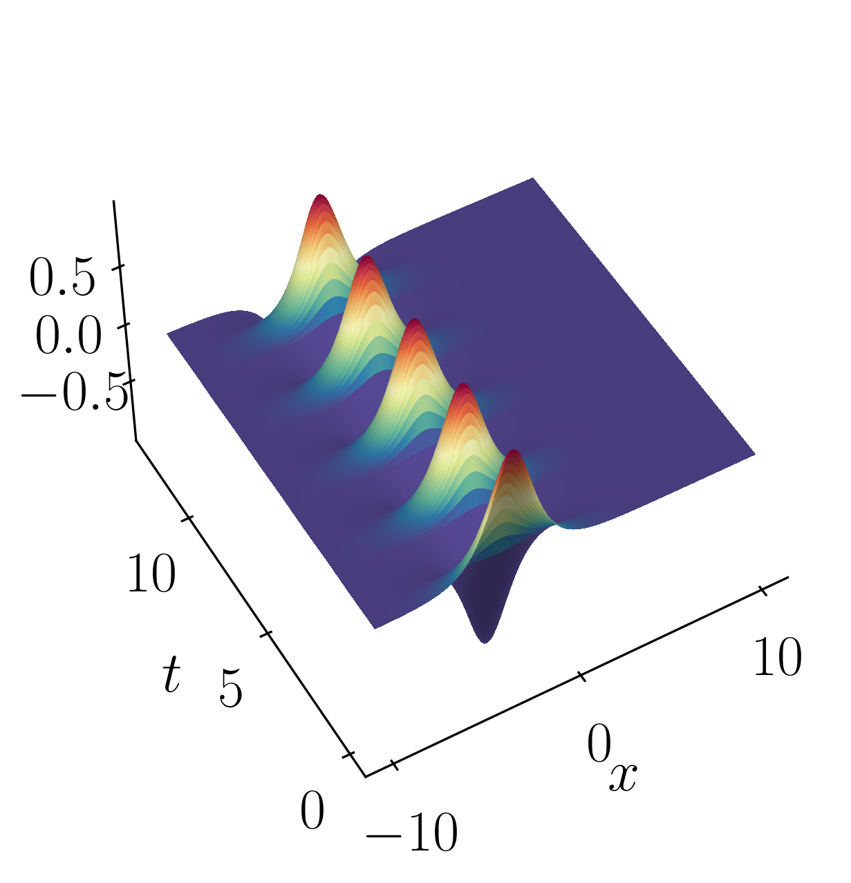
The two signals we’ll be working with are:

where,

and

These signals have frequencies of $\omega_1 = 2.3$ and $\omega_2 = 2.8$, each possessing distinct spatial structures as depicted below:

Let’s kick things off by firing up a Jupyter notebook and importing the necessary modules.

import matplotlib.colors
import matplotlib.pyplot as plt
import numpy as np
import pandas as pd
import scipy as sp
import os
import io
import imageio

%matplotlib inline

plt.rcParams.update({'font.size' : 20, 'font.family' : 'Times New Roman', "text.usetex": True})

After that, let’s proceed to generate the toy signals:

### Define the time and space discretization
xi = np.linspace(-10, 10, 400)
t = np.linspace(0, 4*np.pi, 200)
dt = t[1] - t[0]
[Xgrid, Tgrid] = np.meshgrid(xi, t)

### Create two spatio-temporal signals
def sech(x):
    return 1/np.cosh(x)

f1 = sech(Xgrid+3) * (1*np.exp(1j*2.3*Tgrid))
f2 = (sech(Xgrid)*np.tanh(Xgrid))*(2*np.exp(1j*2.8*Tgrid))

### Combine the signals
f = f1 + f2
X = f.T

Then, you can effortlessly plot the surfaces using matplotlib plotting routines like so:

fig = plt.figure()
ax1 = fig.add_subplot(projection='3d')
ax1.plot_surface(Xgrid, Tgrid, np.real(f), 
                 rstride=1, cstride=1, linewidth=0, antialiased=False, 
                 facecolors=plt.cm.Spectral_r(np.real(f)))
ax1.view_init(50,240)
ax1.set_box_aspect(None, zoom=1)
ax1.set_xlabel(r'$x$')
ax1.set_ylabel(r'$t$')

# make the panes transparent
ax1.xaxis.set_pane_color((1.0, 1.0, 1.0, 0.0))
ax1.yaxis.set_pane_color((1.0, 1.0, 1.0, 0.0))
ax1.zaxis.set_pane_color((1.0, 1.0, 1.0, 0.0))
# make the grid lines transparent
ax1.xaxis._axinfo["grid"]['color'] =  (1,1,1,0)
ax1.yaxis._axinfo["grid"]['color'] =  (1,1,1,0)
ax1.zaxis._axinfo["grid"]['color'] =  (1,1,1,0)

plt.show()

At this stage, since our objective is to apply DMD to our toy dataset, let’s begin by generating the two data matrices as outlined in the DMD algorithm.

# get two views of the data matrix offset by one time step
X1 = np.matrix(X[:, 0:-1])
X2 = np.matrix(X[:, 1:])

Next, utilize the previously defined DMD function to compute the essential diagnostic features of the data. These include the singular values of the data matrix X, the DMD modes Φ, and the continuous-time DMD eigenvalues ω. It’s crucial that these eigenvalues precisely match the underlying frequencies, where their imaginary components correspond to the frequencies of oscillation:

Phi, omega, Lambda, alpha1, b, X_dmd = DMD(X1, X2, 2, dt)
print(omega)

Output:

[-2.71962273e-15+2.8j -7.82921696e-15+2.3j]

Finally, let’s validate the spatial and temporal signals acquired from the rank-2 DMD reconstruction by comparing them with the original signal:

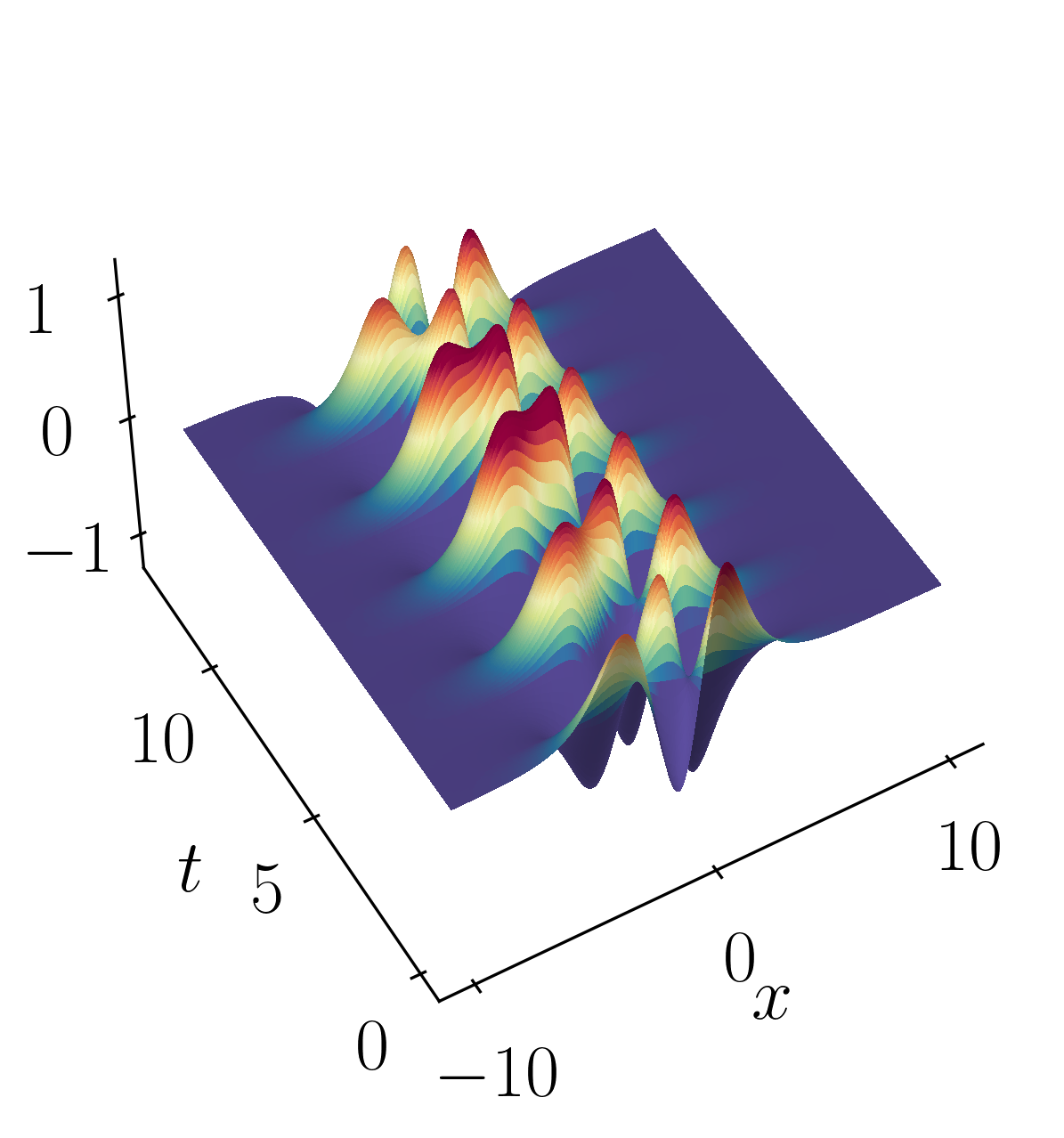
Finally, lets verify the spatial and temporal signals obtained from the rank-2 DMD reconstruction with the original signal.

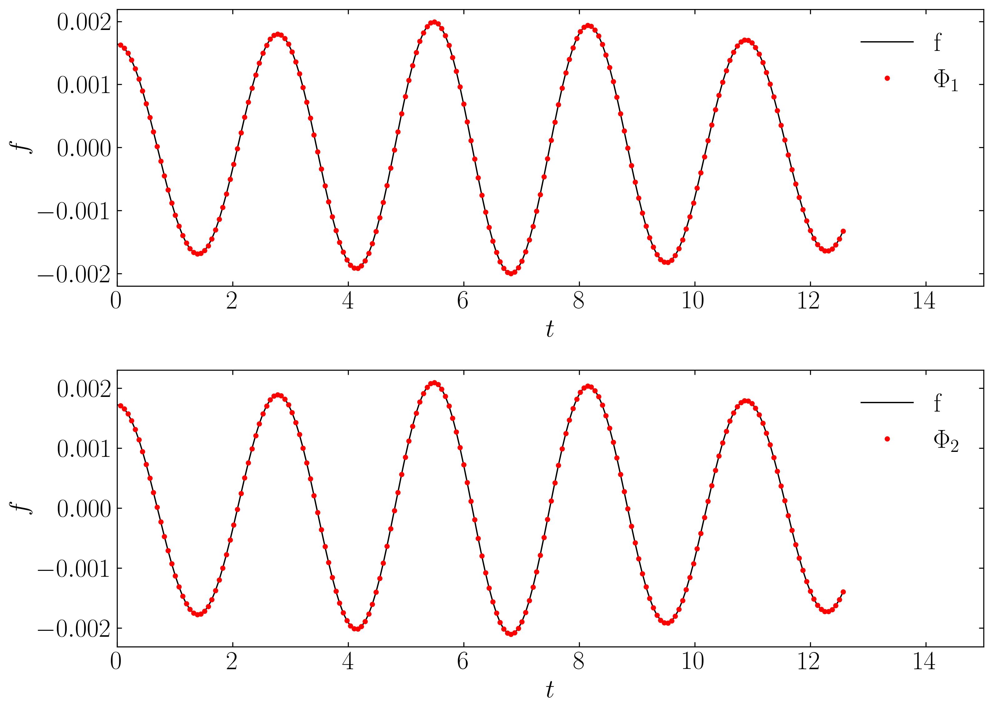
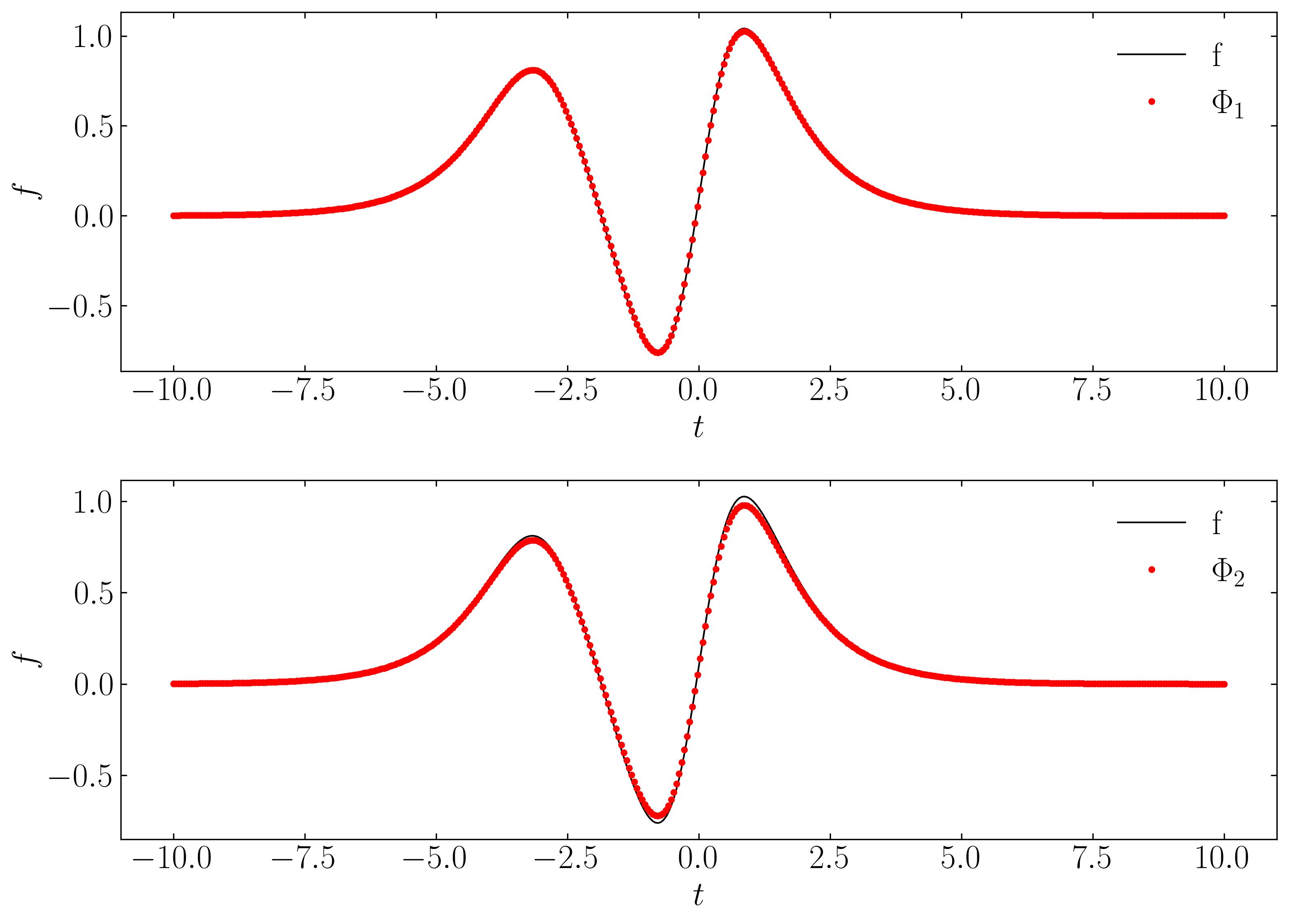
This validation confirms that a rank-2 truncation is suitable. DMD yields results that align precisely (within numerical precision) with the true solution.