Explore Dynamic Mode Decomposition (DMD) with OpenFOAM Simulation Data
Unveiling the secrets of complex systems often requires powerful tools. Enter OpenFOAM, a popular CFD (Computational Fluid Dynamics) software, and Dynamic Mode Decomposition (DMD), a potent data analysis method. This blog post explores the exciting intersection of these two! We’ll explore how DMD can be applied to OpenFOAM simulation data, extracting hidden patterns and dynamics within fluid flows.
In my previous article, I explored how Dynamic Mode Decomposition (DMD) has been applied and pioneered in the field of applied fluid dynamics, playing a crucial role in the identification and analysis of spatio-temporal coherent structures. We covered the fundamentals of DMD, its relationship with Singular Value Decomposition (SVD) and Proper Orthogonal Decomposition (POD)—other modal decomposition methods I’ve discussed earlier—and applied the DMD algorithm to the publicly available dataset of flow around a circular cylinder.
In this article, we will focus on the open-source Computational Fluid Dynamics powerhouse, OpenFOAM. We’ll take a practical approach, using the Python programming language to directly analyze field data extracted from OpenFOAM time directories and compute Dynamic Mode Decomposition on the data.
Let’s begin!
Prerequisites
Setting Up the Case
In order to explore Dynamics Mode Decomposition (DMD) using a combination of OpenFOAM and Python, our focus will center on examining the dynamics of a two-dimensional flow around a square cylinder at a Reynolds number of 100. This exploration will entail simulating the flow through Direct Numerical Simulations (DNS) using OpenFOAM. The configuration of this case closely follows the guidelines outlined by Bai and Alam (2018) for reference. You can find detailed instructions in their work.
Refer to the my previous article to setup a case following the criterions defined by Bai and Alam (2018).
Verify that your case adheres to the specifications outlined in the reference and includes multiple time directories (snapshots) resembling the format below:
7470.000000116633  7560.000000118597  7650.000000120562  7740.250000122532  7831.250000124518  7922.250000126504
7470.750000116649  7561.750000118635  7651.000000120584  7742.00000012257   7833.000000124556  7924.000000126543
...
7547.75000011833   7638.750000120316  7728.000000122264  7819.000000124251  7910.000000126237  constant
7549.500000118368  7640.500000120354  7729.750000122302  7820.750000124289  7911.750000126275  postProcessing
7551.250000118406  7642.250000120393  7731.500000122341  7822.500000124327  7913.500000126313  system
PRO TIP: Ensure a minimum of 256 snapshots are captured for your data.
Visualization Case Setup
For data visualization purposes, we will establish a separate directory for a second case setup. Begin by duplicating the 0, constant, and system files from your original case into a new directory named visualizationCase. Additionally, within this new directory, create a time directory named 1 to facilitate the organization of your data.
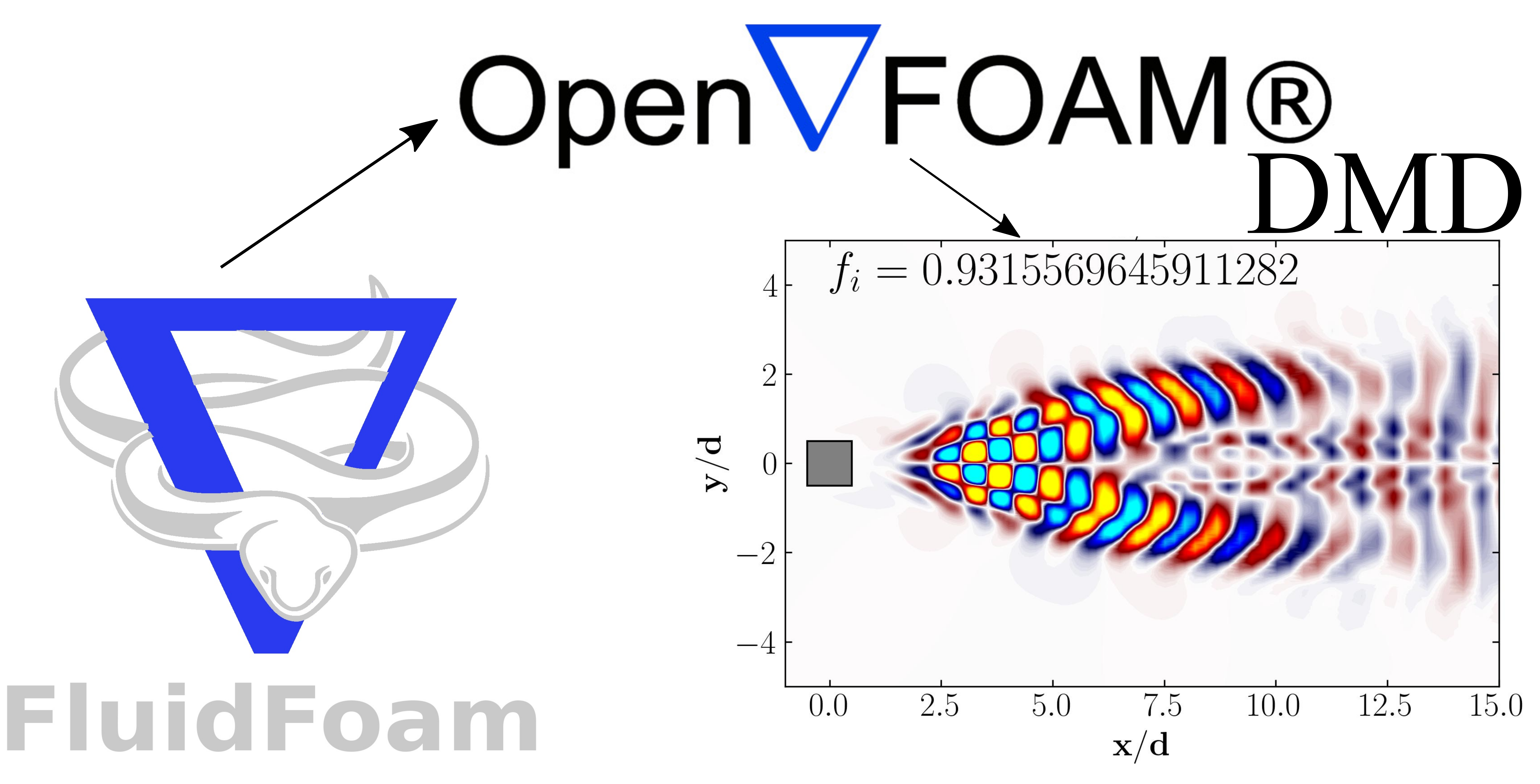
Utilizing FluidFoam
Our exploration heavily relies on a Python package called fluidfoam. This specialized package is crafted specifically for OpenFOAM post-processing tasks. Fluidfoam streamlines intricate operations such as extracting velocity and pressure data from simulations, seamlessly managing OpenFOAM-specific data structures, and facilitating insightful visualizations with minimal complexity.
For instance, extracting the velocity field from within OpenFOAM is simplified using fluidfoam. Here’s an example code snippet:
# import readvector function from fluidfoam package
from fluidfoam import readvector
vel = readvector('Path/To/Your/Case', time_name='latestTime', name='U', structured=False)
In this snippet, vel represents the velocity vector imported into Python from your OpenFOAM case. It reads the latest available time (time_name='latestTime') and any specified fields (name='U'). Other available fields include UMean, UPrime2Mean, p, pMean, etc. The variable vel produces a numpy ndarray of size (3 x NumberOfCells). Transposing the data is necessary to obtain a (NumberOfCells x 3) array:
new_vel = np.reshape(vel.T,(216000,1), order='F')
Here, vel.T denotes the transpose of the velocity vector array, and order='F' ensures the maintenance of element order. 'F' specifies Fortran-like index order, where the first index changes fastest and the last index changes slowest.
After matrix manipulation, the reshaped velocity array can be transformed back to its original format (transpose form) using:
new_vel = np.reshape(new_vel, (72000,3), order='F')
This reshaped matrix retains the same mesh order as the original field and can be effortlessly integrated into OpenFOAM cases for post-processing via tools like Tecplot or ParaView.
Dynamic Mode Decomposition (DMD)
Let’s kick off by launching a Jupyter notebook and importing the essential modules:
import matplotlib.colors
import matplotlib.pyplot as plt
import numpy as np
import pandas as pd
import fluidfoam as fl ### Most Important
import scipy as sp
from matplotlib.colors import ListedColormap
import os
import io

%matplotlib inline

plt.rcParams.update({'font.size' : 18, 'font.family' : 'Times New Roman', "text.usetex": True})
Step 1: Setting Up Paths
Begin by assigning paths to your case directory and the folder where you intend to store your data:
Path = 'E:/Blog_Posts/OpenFOAM_POD/Square_Cylinder_Laminar/'
save_path = 'E:/Blog_Posts/OpenFOAM/ROM_Series/Post29/'
Step 2: Extracting Time Directories as a List
Navigate to your OpenFOAM case within a Linux terminal on WSL or Ubuntu. First, within OpenFOAM, execute the command:
foamListTimes | tee times.txt
This command generates a text file named times.txt, listing all the time directory names.
In Python, convert the text file into a list using the following code:
Times = open(Path + 'times.txt').read().splitlines()
Snapshots = len(Times)
print(Snapshots)
### Output
### 256
This method results in Times being a list of strings. For instance, Times[0] = 'xxxx' (a string that can be directly read into the subsequent line of code). The output, indicating the number of snapshots, should match the number of time directories saved in your case.
Step 3: Reading a Velocity Vector Field
Let’s attempt to read a velocity field from OpenFOAM into Python using fluidfoam.
vel = fl.readvector(Path, time_name='latestTime', name='U', structured=False)
columns, rows = np.shape(vel.T)
print(columns, rows)
### Output
### 95868 3
Successfully, we’ve imported a vector field from the OpenFOAM case into Python. Verify and assign the shape of the vector field to determine the number of rows and columns in your dataset, which will prove useful later.
Note: Here, columns correspond to the total number of data points in the internal mesh, while rows represent the velocity components (u, v, and w).
Step 4: Assembling the Data Matrices
At this stage, we need to assemble two crucial data matrices. First, the mean-centered dataset required to compute POD prior to DMD, and second, the data matrix containing instantaneous velocity field information for all snapshots. These correspond to the B and X matrices in our algorithm.
B = np.zeros((columns*rows,Snapshots)) # Matrix to store the fluctuating velocity field
X = np.zeros((columns*rows,Snapshots)) # Matrix to store the velocity field

# Reading the mean velocity field
Mean_vel1 = fl.readvector(Path, time_name=str(Times[0]), name='UMean', structured=False)
new_Mean_Vel1 = np.reshape(Mean_vel1.T,(columns*rows,1), order='F')

for i in np.arange(0,Snapshots):
    vel1 = fl.readvector(Path, time_name=str(Times[i]), name='U', structured=False)
    new_vel1 = np.reshape(vel1.T,(columns*rows,1), order='F')
    MC = new_vel1 - new_Mean_Vel1
    B[:,i:i+1] = MC
    X[:,i:i+1] = new_vel1

np.save(save_path + 'B.npy', B)
np.save(save_path + 'X.npy', X)
Since we’ve run the case until it reached statistical stability, we can obtain the mean velocity (UMean) using OpenFOAM function objects and then utilize it here to derive the mean-centered matrix, B.
Step 5: Apriori POD Analysis
Lets first compute Proper Orthogonal Decomposition (POD) of the flow field. This will aid in determining the appropriate r-rank approximation needed for DMD. Remember, DMD relies on Singular Value Decomposition (SVD) reduction to execute a low-rank truncation of the data.
### POD Analysis

### Data Matrix = B (Mean-removed Matrix)
### Mean-removed Matrix
B_mean = np.mean(B, axis = 1)
Y = B - B_mean[:,np.newaxis]

### Covariance Matrix
C = np.dot(Y.T, Y)/(Y.shape[1]-1)

### SVD of Covariance Matrix
U, S, V = np.linalg.svd(C)

### POD modes
Phi = np.dot(Y, U)

### Temporal coefficients
a = np.dot(Phi.T, Y)
Following this, let’s directly examine the energy content of the initial POD modes to determine the r-rank approximation needed for DMD.
Energy = np.zeros((len(S),1))
for i in np.arange(0,len(S)):
    Energy[i] = S[i]/np.sum(S)

X_Axis = np.arange(Energy.shape[0])
heights = Energy[:,0]

fig, axes = plt.subplots(1, 2, figsize = (12,4))
ax = axes[0]
ax.plot(Energy, marker = 'o', markerfacecolor = 'none', markeredgecolor = 'k', ls='-', color = 'k')
ax.set_xlim(0, 20)
ax.set_xlabel('Modes')
ax.set_ylabel('Energy Content')

ax = axes[1]
cumulative = np.cumsum(S)/np.sum(S)
ax.plot(cumulative, marker = 'o', markerfacecolor = 'none', markeredgecolor = 'k', ls='-', color = 'k')
ax.set_xlabel('Modes')
ax.set_ylabel('Cumulative Energy')
ax.set_xlim(0, 20)

# plt.savefig(save_path + 'Energy.jpeg', dpi = 300, bbox_inches = 'tight')

plt.show()
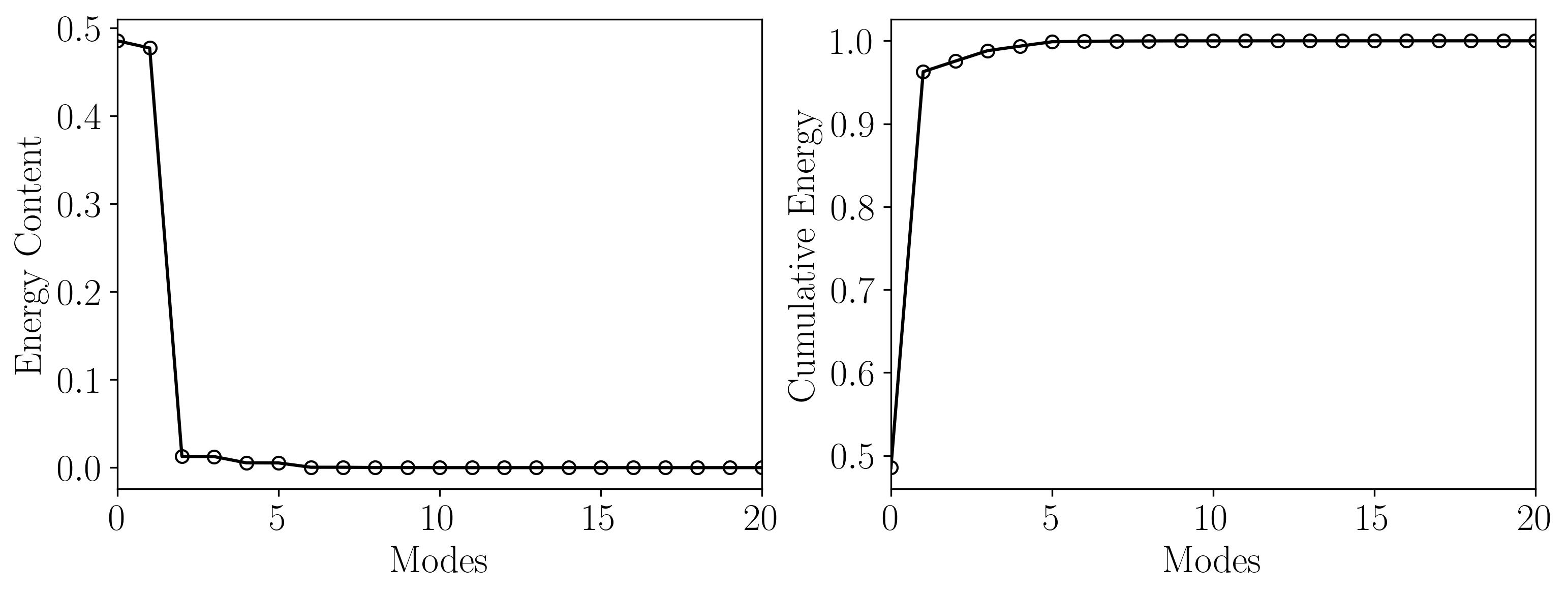
This analysis reveals that the first 21 POD modes capture approximately 99.9% of the total energy. Therefore, a rank-21 approximation for DMD will suffice!
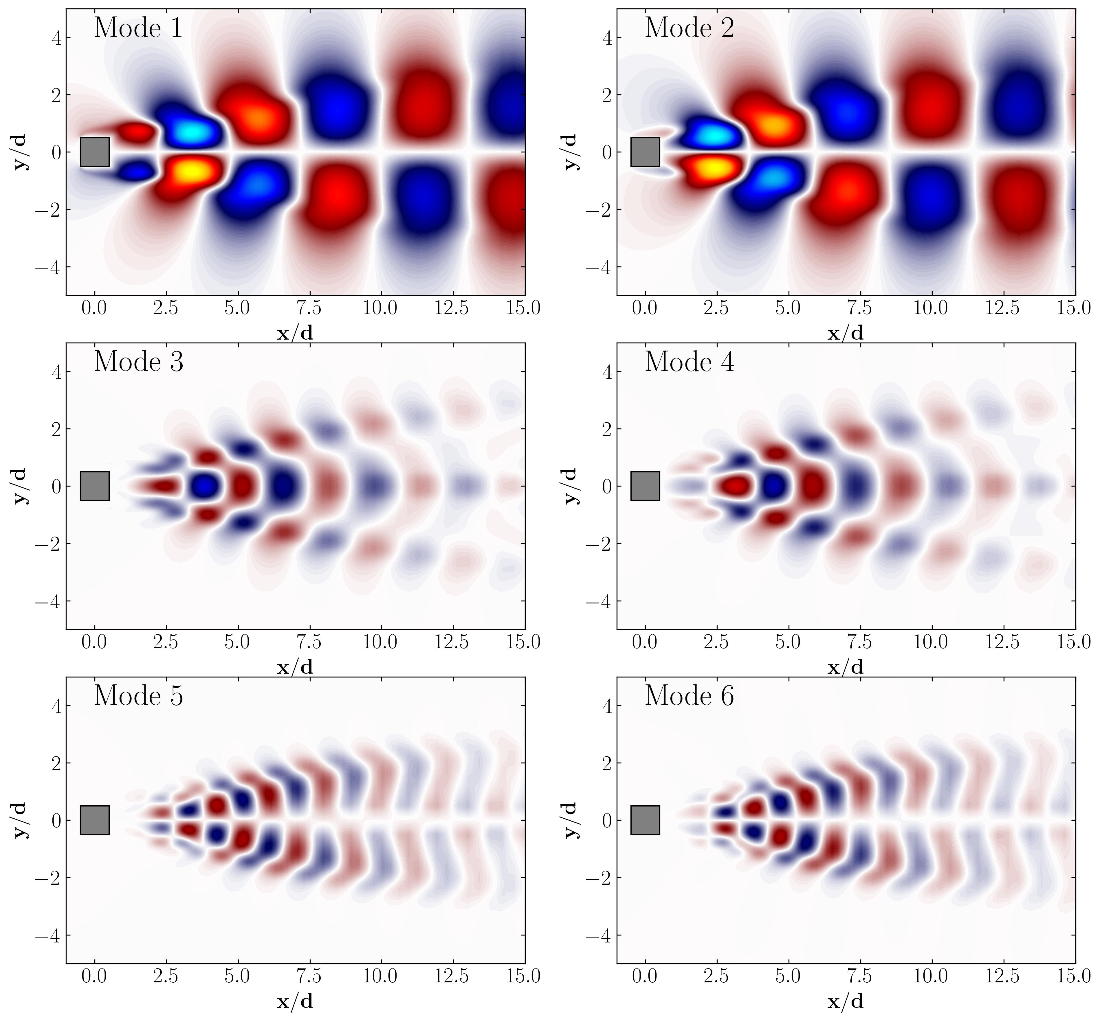
Finally, you can extract the POD modes and visualize them using Python:
Step 6: DMD Algorithm
We will be using a DMD function to extract all the necessary information from the two data matrices we input to it. For reference, here is the DMD function:
def DMD(X1, X2, r, dt):
    U, s, Vh = np.linalg.svd(X1, full_matrices=False)
    ### Truncate the SVD matrices
    Ur = U[:, :r]
    Sr = np.diag(s[:r])
    Vr = Vh.conj().T[:, :r]

    ### Build the Atilde and find the eigenvalues and eigenvectors
    Atilde = Ur.conj().T @ X2 @ Vr @ np.linalg.inv(Sr)
    Lambda, W = np.linalg.eig(Atilde)

    ### Compute the DMD modes
    Phi = X2 @ Vr @ np.linalg.inv(Sr) @ W

    omega = np.log(Lambda)/dt ### continuous time eigenvalues

    ### Compute the amplitudes

    alpha1 = np.linalg.lstsq(Phi, X1[:, 0], rcond=None)[0] ### DMD mode amplitudes

    b = np.linalg.lstsq(Phi, X2[:, 0], rcond=None)[0] ### DMD mode amplitudes

    ### DMD reconstruction
    time_dynamics = None
    for i in range(X1.shape[1]):
        v = np.array(alpha1)[:,0]*np.exp( np.array(omega)*(i+1)*dt)
        if time_dynamics is None:
            time_dynamics = v
        else:
            time_dynamics = np.vstack((time_dynamics, v))
    X_dmd = np.dot( np.array(Phi), time_dynamics.T)

    return Phi, omega, Lambda, alpha1, b, X_dmd
To use this, lets first obtain our time-shifted data matrices:
# get two views of the data matrix offset by one time step
X1 = np.matrix(X[:, 0:-1])
X2 = np.matrix(X[:, 1:])
And define the rank of approximation and the time-step:
r = 21
dt = 0.01*175
Then simply use the function above to compute DMD:
Phi, omega, Lambda, alpha1, b, X_dmd = DMD(X1, X2, r, dt)
Now, before diving into visualization, let’s examine the distribution of eigenvalues extracted from the DMD algorithm. Specifically, we need to understand the dynamic behavior of the DMD modes we’ve identified. To do this, plot a simple unit circle and overlay the scatter plot of the real versus imaginary eigenvalues onto it by:
theta = np.linspace( 0 , 2 * np.pi , 150 )
radius = 1
a = radius * np.cos( theta )
b = radius * np.sin( theta )

fig, ax = plt.subplots()

ax.scatter(np.real(Lambda), np.imag(Lambda), color = 'r', marker = 'o', s = 100)
ax.plot(a, b, color = 'k', ls = '--')

ax.set_xlabel(r'$\Lambda_r$')
ax.set_ylabel(r'$\Lambda_i$')

ax.set_aspect('equal')

plt.show()
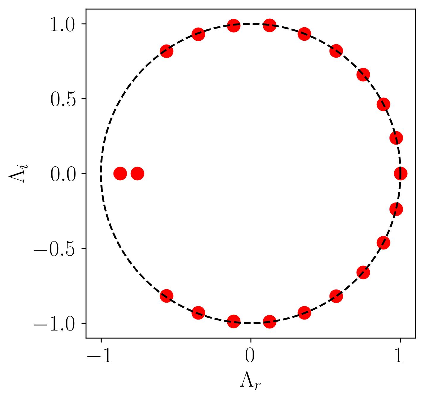
In this plot, all points lie on the unit circle, indicating that the modes neither grow nor decay, signifying stable DMD modes. Additionally, we observe two outliers where the eigenvalues reside inside the unit circle, indicating that these dynamic modes are decaying.
Data visualization
To prepare the DMD modes for visualization, we need to save them to an OpenFOAM native format file, which can then be read into Tecplot or ParaView. First, let’s create two text files named header.txt and footer.txt. Open any vector field file from your time directories and copy the header and footer sections into these text files. Save them in the Path file location.
The contents of the header.txt file should be as follows:
/*--------------------------------*- C++ -*----------------------------------*\
| =========                 |                                                 |
| \\      /  F ield         | OpenFOAM: The Open Source CFD Toolbox           |
|  \\    /   O peration     | Version:  2312                                  |
|   \\  /    A nd           | Website:  www.openfoam.com                      |
|    \\/     M anipulation  |                                                 |
\*---------------------------------------------------------------------------*/
FoamFile
{
    version     2.0;
    format      ascii;
    arch        "LSB;label=32;scalar=64";
    class       volVectorField;
    location    "7470.750000116649";
    object      U;
}
// * * * * * * * * * * * * * * * * * * * * * * * * * * * * * * * * * * * * * //

dimensions      [0 1 -1 0 0 0 0];

internalField   nonuniform List<vector>
95868
(
And the contents of the footer.txt file should be as follows:
)
;

boundaryField
{
    INLET
    {
        type            fixedValue;
        value           uniform (0.015 0 0);
    }
    OUTLET
    {
        type            zeroGradient;
    }
    TOP
    {
        type            slip;
    }
    BOTTOM
    {
        type            slip;
    }
    SIDE1
    {
        type            slip;
    }
    SIDE2
    {
        type            slip;
    }
    PRISM
    {
        type            noSlip;
    }
}


// ************************************************************************* //
Now, let’s read the header and footer files into Python:
# For Header
with open(Path + 'header.txt') as f:
    header="".join([f.readline() for i in range(23)])  ### 22 is number of rows

# For Footer
with open(Path + 'footer.txt') as f:
    footer="".join([f.readline() for i in range(39)])
We can now save the POD modes into OpenFOAM-readable files by combining the header and footer files with the calculated POD modes:
saveTime = 'E:/Blog_Posts/OpenFOAM_POD/TestCase_DMD/'

### Save the DMD Modes
for i in np.arange(0,len(Lambda)):
    Mode = np.reshape(np.real(Phi[:,i]), (columns,rows), order='F')
    np.savetxt(saveTime + 'Mode' + str(i+1), Mode, fmt='(%s %s %s)', header=header, footer=footer, comments='')

### Save the Reconstructed flow field
First = np.reshape(np.real(X_dmd[:,0]), (columns,rows), order='F')
np.savetxt(saveTime + 'XDMD', First, fmt='(%s %s %s)', header=header, footer=footer, comments='')
Don’t forget to rename the object within each of these files to the respective names for simplicity, as follows:
object Mode1;
Finally, after changing the object name, copy these files into the time directory of visualizationCase we created earlier.
Results
To visualize the results, we can employ either ParaView or Tecplot for post-processing. However, another method involves utilizing the OpenFOAM vtk file extractions. While the first method is straightforward, let’s explore the second one instead.
Begin by utilizing the surfaces function object executed through the command-line. Set up a surfaces file within the system directory as shown below:
surfaces
{
    type            surfaces;
    libs            ("libsampling.so");
    writeControl   	timeStep;
    writeInterval   10;

    surfaceFormat   vtk;

    fields          (p U XDMD Mode1 Mode2 Mode3 Mode4 Mode5 Mode6 Mode7 Mode8 Mode9 Mode10 Mode11 Mode12 Mode13 Mode14 Mode15 Mode16 Mode17 Mode18 Mode19 Mode20);

    interpolationScheme cellPoint;

    surfaces
    {
        zNormal
        {
            type        cuttingPlane;
            point       (0 0 0.05);
            normal      (0 0 1);
            interpolate true;
        }
    };
};
Now, let’s proceed to extract the data using the postProcess utility with the command:
postProcess -func surfaces
Executing this command will generate a file named surfaces within the postProcessing directory, containing the surface field in a vtk file, as shown below:
surfaces/
└── 1
    └── zNormal.vtp
This vtk file can be readily opened in ParaView or VisIt for visualization. However, today we will visualize these fields in Python using the PyVista module. PyVista is a powerful tool for 3D data visualization, serving as an interface for the Visualization Toolkit (VTK). With PyVista, one can easily read and extract data from a vtk file. In your Jupyter file, start by importing the module:
import pyvista as pv
Then set the path variables:
PathToSurfaces = 'E:/Blog_Posts/OpenFOAM_POD/TestCase_DMD/postProcessing/surfaces/1/'
Files = os.listdir(PathToSurfaces)
Now, extract the VTK file using the PyVista module:
Data = pv.read(PathToSurfaces + Files[0])
grid = Data.points
x = grid[:,0]
y = grid[:,1]
z = grid[:,2]
rows, columns = np.shape(grid)
print('rows = ', rows, 'columns = ', columns)
Check which arrays are available within this extracted vtk file:
print(Data.array_names)
Output:
['TimeValue', 'p', 'Mode1', 'Mode10', 'Mode11', 'Mode12', 'Mode13', 'Mode14', 'Mode15', 'Mode16', 'Mode17',
'Mode18', 'Mode19', 'Mode2', 'Mode20', 'Mode3', 'Mode4', 'Mode5', 'Mode6', 'Mode7', 'Mode8', 'Mode9', 'U',
'XDMD']
Extract the DMD modes from the Data:
Velocity = Data['U']
Pressure = Data['p']
Mode1 = Data['Mode1']
Mode2 = Data['Mode2']
Mode3 = Data['Mode3']
Mode4 = Data['Mode4']
Mode5 = Data['Mode5']
Mode6 = Data['Mode6']
Mode7 = Data['Mode7']
Mode8 = Data['Mode8']
Mode9 = Data['Mode9']
Mode10 = Data['Mode10']
Mode11 = Data['Mode11']
Mode12 = Data['Mode12']
Mode13 = Data['Mode13']
Mode14 = Data['Mode14']
Mode15 = Data['Mode15']
Mode16 = Data['Mode16']
Mode17 = Data['Mode17']
Mode18 = Data['Mode18']
Mode19 = Data['Mode19']
Mode20 = Data['Mode20']
XDMD = Data['XDMD']
Then simply plot the DMD modes using simple matplotlib routines:
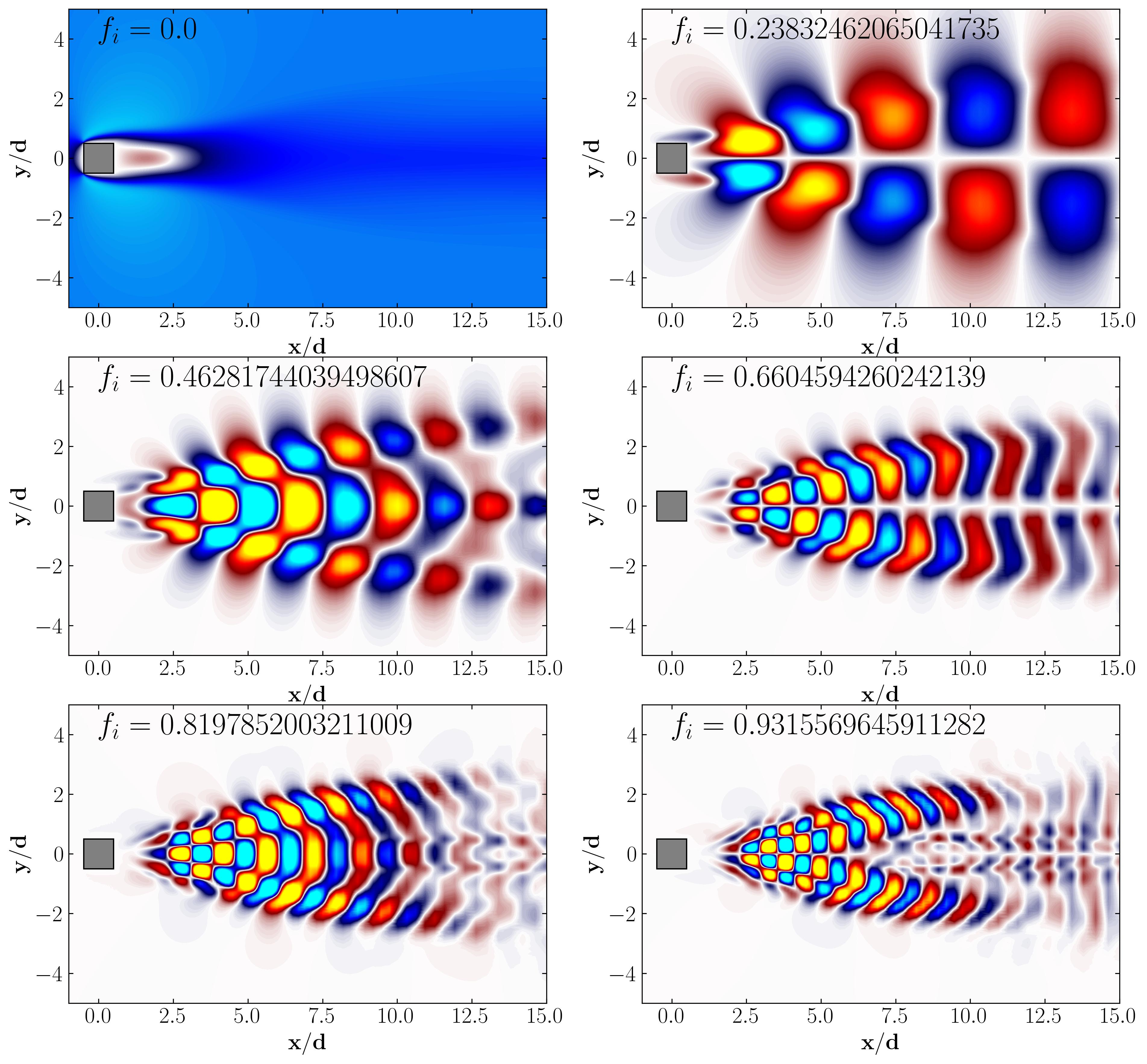
In conclusion, in this article, we explored how to apply the Dynamic Mode Decomposition algorithm directly to snapshot data retrieved from OpenFOAM. In the next article, we’ll examine another method of computing DMD using OpenFOAM data, this time utilizing an extracted slice dataset from the simulation. This approach will allow us to work with larger datasets, more snapshots, and lesser spatial degrees of freedom.
Enjoy Reading This Article?
Here are some more articles you might like to read next: