Unlocking Insights: Exploring Singular Value Decomposition (SVD) and its Dynamic Applications

Delving deep into the realm of Singular Value Decomposition (SVD) and its impactful applications, join me as I unravel the versatility of SVD, from its pivotal role in image compression to its effectiveness in linear and multilinear regression. Explore how SVD uncovers hidden patterns in data, enabling informed decision-making and empowering data analysis across various domains.

In this article, I will explore concrete examples that illuminate the versatility and power of SVD across different domains, from image compression to linear regression and beyond. SVD, a cornerstone of linear algebra, lies at the heart of numerous data analysis and machine learning techniques. Its ability to reveal underlying structures in data makes it indispensable for tasks ranging from dimensionality reduction to pattern recognition. By decomposing complex datasets into simpler components, SVD empowers us to extract meaningful insights and make informed decisions. In this post, we’ll dive into two illustrative examples of SVD in action: image compression and linear regression. Through these examples, we’ll demonstrate how SVD can be leveraged to solve real-world problems and enhance the efficiency and effectiveness of data analysis workflows. Let’s dive in!

Image compression

To demonstrate the concept of matrix approximation using Singular Value Decomposition (SVD), let’s consider a simple example of image compression. Large datasets often exhibit underlying patterns that allow for efficient low-rank representations, making them inherently compressible. Images, in particular, provide an intuitive example of this compressibility, as they can be represented as matrices of pixel values.

As an example, let’s work with an image of Dr. Richard Feynman, a physics hero. We’ll import this image into a Jupyter notebook using Python. Here’s how you can do it:

### Import modules
import numpy as np
import matplotlib.pyplot as plt
from matplotlib import colors
import math as mt
from numpy import linalg as LA
plt.rcParams.update({'font.size' : 22, 'font.family' : 'Times New Roman', "text.usetex": True})

mat = plt.imread('Richard_Feynman.png')

fig, ax = plt.subplots()
p = ax.imshow(mat, cmap = 'gray')
plt.show()

This code reads the image file and displays it using Matplotlib. Make sure to adjust the file path accordingly to locate the image file on your system.

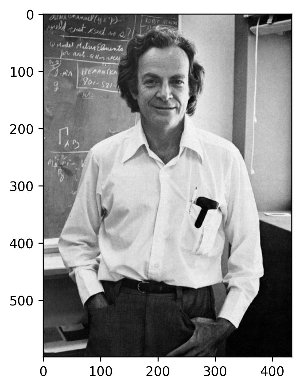
To analyze the size of the image in terms of the number of pixels, we can use the .shape attribute of the image array. This attribute returns a tuple containing the dimensions of the image array, representing its height and width in pixels. Here’s how you can do it:

mat.shape

### Output
### (599, 434)

This observation reveals that the image portraying Dr. Feynman comprises a total of 599 x 434 pixels. Now, let’s delve into the realm of Singular Value Decomposition (SVD) by applying it to the matrix encapsulating the pixel data of this image.

### SVD
U, s, VT = LA.svd(mat)

### Form diagonal matrix
Sigma = np.zeros((mat.shape[0], mat.shape[1]))
Sigma[:min(mat.shape[0], mat.shape[1]), :min(mat.shape[0], mat.shape[1])] = np.diag(s)

Plot the singular or eigen values and the cummulative eigenvalues for this image by

cumulative = np.cumsum(s)/np.sum(s)

fig, ax = plt.subplots()

ax.semilogy(s, marker = 'o', markerfacecolor = 'none', markeredgecolor = 'k', ls='-', color = 'k')

ax.set_xlabel(r'$n$')
ax.set_ylabel('Singular Values,' + r'$\sigma_n$')
ax.xaxis.set_tick_params(direction='in', which='both')
ax.yaxis.set_tick_params(direction='in', which='both')
ax.xaxis.set_ticks_position('both')
ax.yaxis.set_ticks_position('both')

plt.show()

fig, ax = plt.subplots()

ax.plot(cumulative, marker = 'o', markerfacecolor = 'none', markeredgecolor = 'k', ls='-', color = 'k')

ax.plot(40, 0.725, marker = 'o', markerfacecolor = 'r', c='r', markersize = 10)
ax.text(50, 0.7, r'$r = 40$', fontsize = 20, color = 'r')

ax.plot(80, 0.825, marker = 'o', markerfacecolor = 'r', c='r', markersize = 10)
ax.text(95, 0.80, r'$r = 80$', fontsize = 20, color = 'r')

ax.plot(120, 0.885, marker = 'o', markerfacecolor = 'r', c='r', markersize = 10)
ax.text(135, 0.86, r'$r = 120$', fontsize = 20, color = 'r')

ax.plot(240, 0.965, marker = 'o', markerfacecolor = 'r', c='r', markersize = 10)
ax.text(240, 0.91, r'$r = 240$', fontsize = 20, color = 'r')

ax.set_xlabel(r'$n$')
ax.set_ylabel(r'$\sum\sigma_n$')
ax.xaxis.set_tick_params(direction='in', which='both')
ax.yaxis.set_tick_params(direction='in', which='both')
ax.xaxis.set_ticks_position('both')
ax.yaxis.set_ticks_position('both')

plt.show()

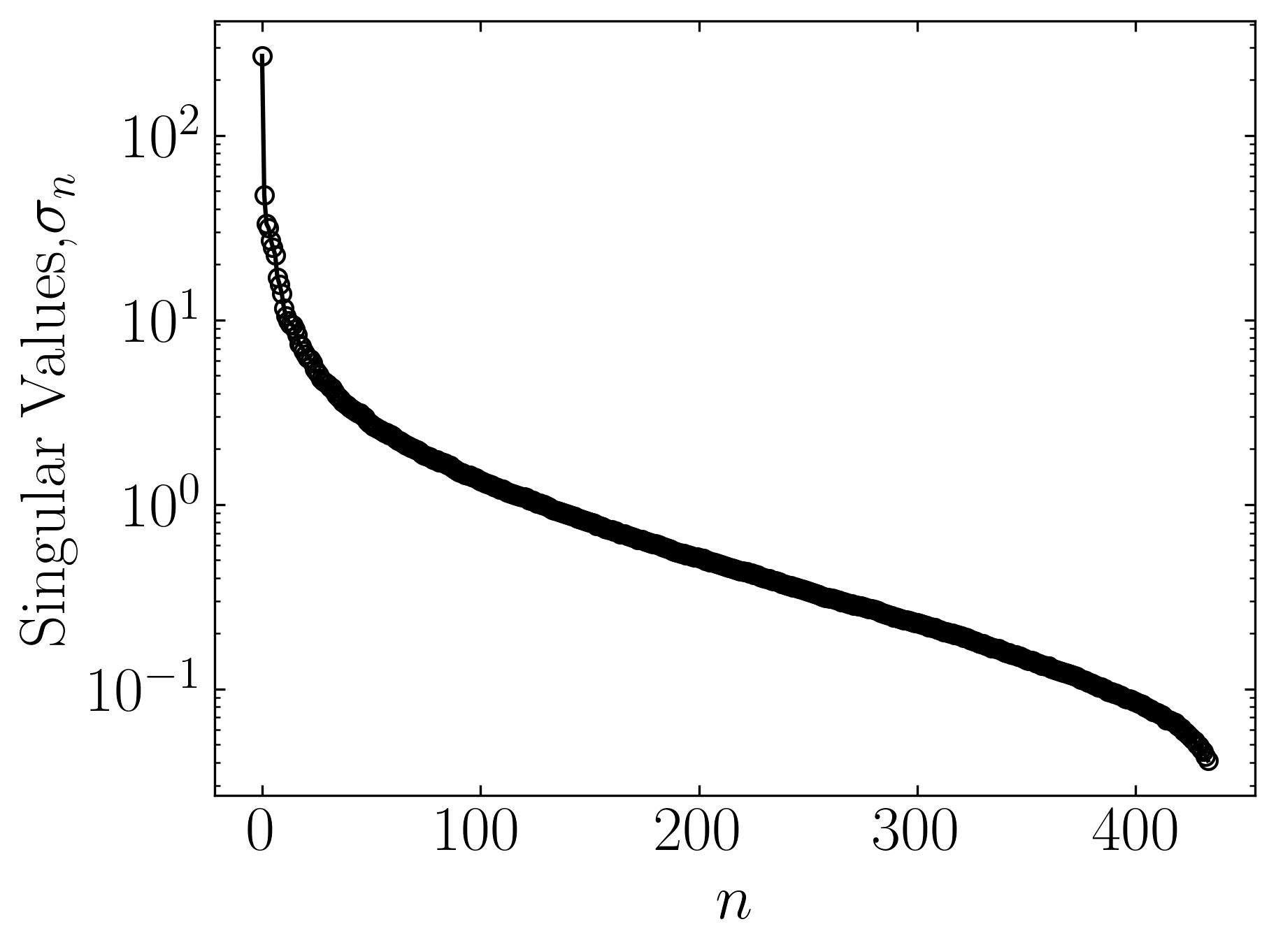
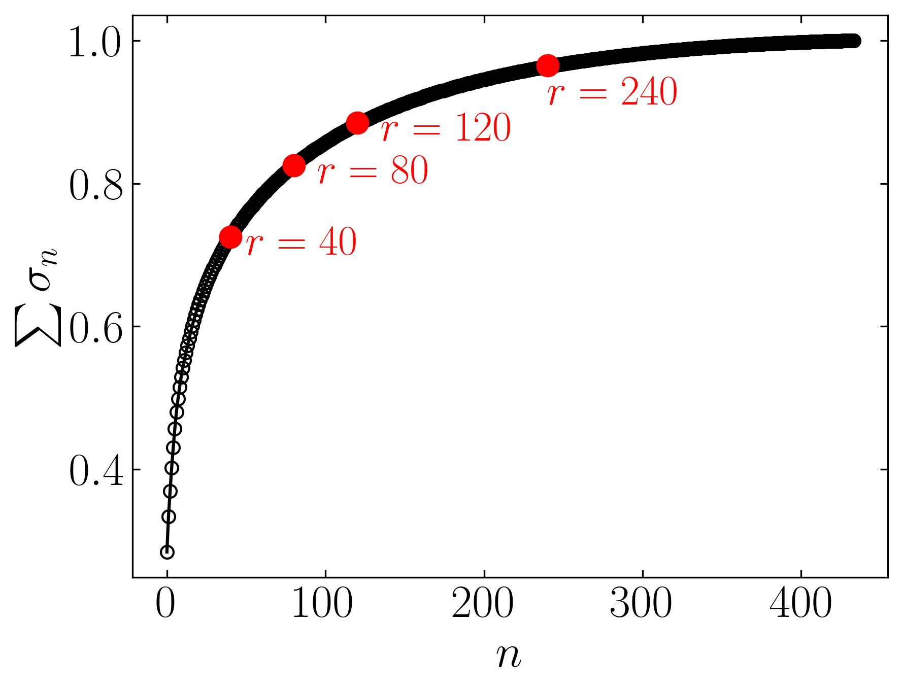
The initial figure to the left arranges the eigenvalues in order based on the number of snapshots, corresponding to the horizontal pixels. Meanwhile, the subsequent figure illustrates the cumulative sum of eigenvalues against the number of snapshots (n). Additionally, this graph highlights the ranks of 40, 80, 120, and 240, correlating to approximately 9%, 18%, 28%, and 55% compression in the image.

To obtain approximations for these ranks, one can readily execute the following:

### Rank
k = 40 # 80, 120, 240

### Approximation
mat_approx = U[:, :k] @ Sigma[:k, :k] @ VT[:k, :]

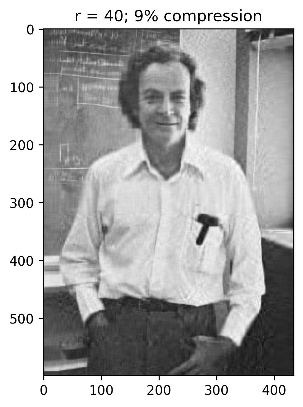
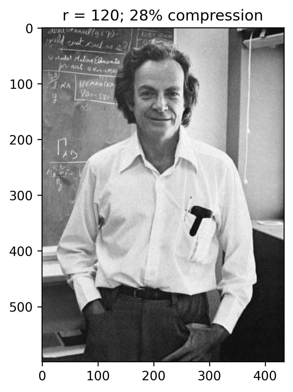
With a rank (r) of 240, the reconstructed image appears notably accurate, with the singular values encompassing nearly 55% of the image variance. This truncation via Singular Value Decomposition (SVD) effectively compresses the original image, necessitating the storage of solely the first 240 columns of U and V matrices, along with the first 240 diagonal elements of the S matrix in U_Hat, S_Hat, and V_Hat. Consequently, SVD serves as a pivotal tool for data compression, preserving the essence of the data while significantly reducing the matrix’s size.

Least-squares and Regression

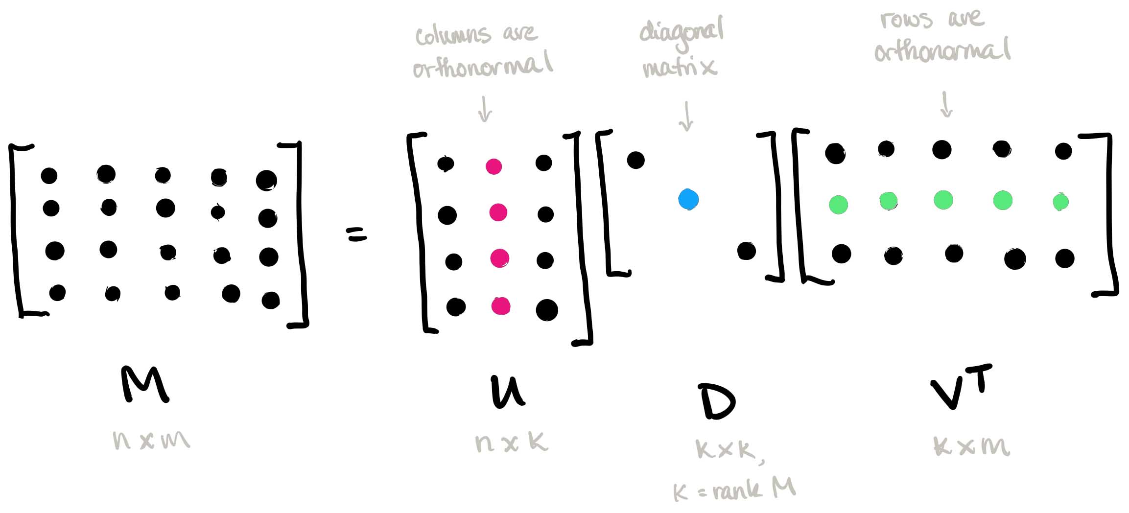
Singular Value Decomposition (SVD) plays a crucial role in various data science applications, particularly in regression and least-square fitting methods. Many real-world scenarios can be modeled as linear systems of equations, represented as:

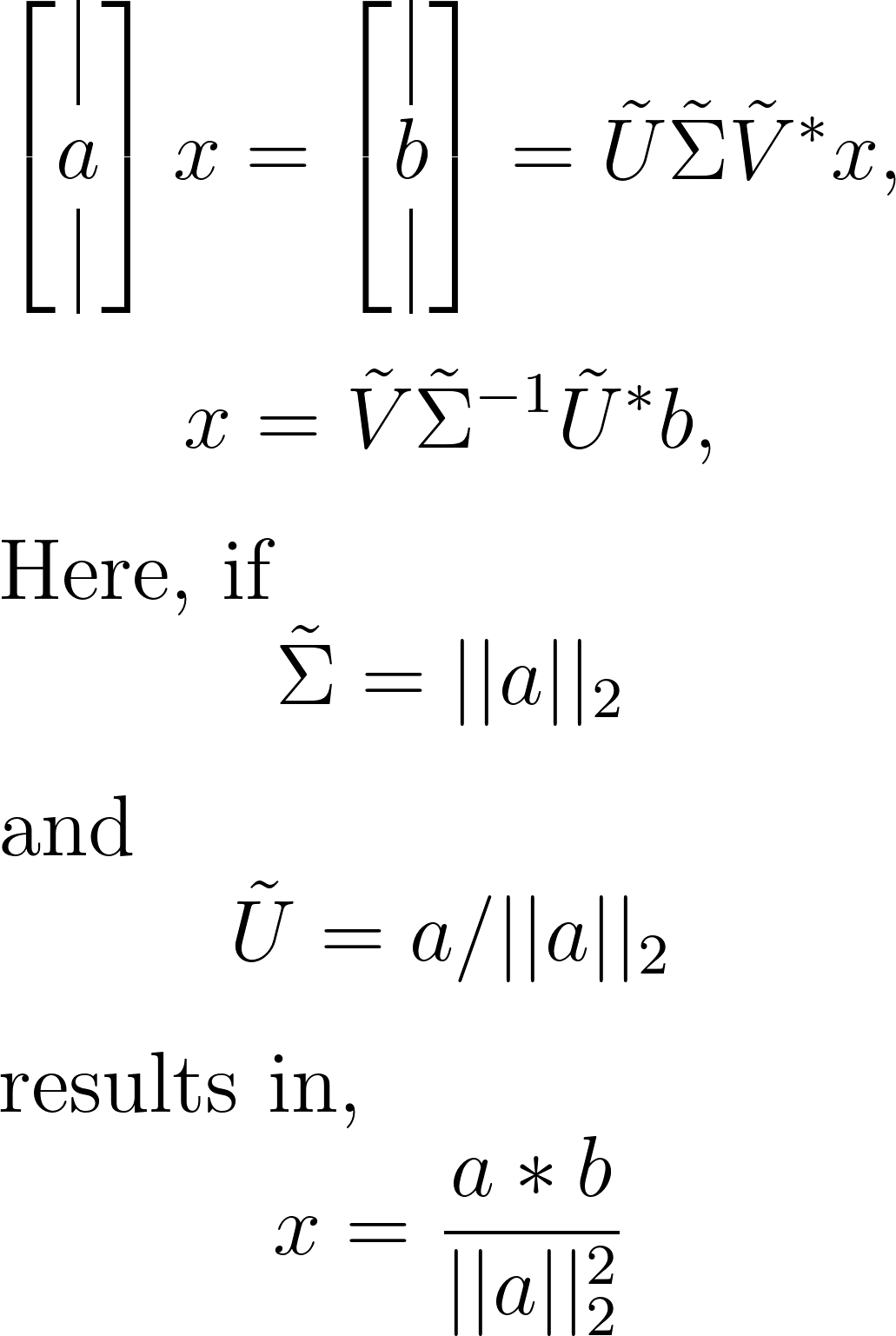
Here, the matrix A and vector b are known, while the vector x represents the unknowns. Matrix A typically has m rows and n columns. When A is square (m = n), a unique solution exists for every b. However, situations arise where A is singular or rectangular (m > n, m < n, or m = n = 1), leading to scenarios with one, none, or infinite solutions for x, depending on the specific A and b. We’ll focus on overdetermined systems, where A is a tall, skinny matrix (m >> n).

In overdetermined systems lacking solutions, we often seek the solution x that minimizes the sum-squared error, $\Vert$ $Ax - b$ $\Vert$ $_2^2$, known as the least-squares solution. This method also minimizes $\Vert$ $Ax - b$ $\Vert$ $_2$ (L2 Norm), crucial in scenarios with infinitely many solutions, where we aim to find the solution of x with the minimum L2 norm ($\Vert$x$\Vert$$_2$) to satisfy Ax = b, termed the minimum-norm solution. SVD proves indispensable for optimizing such problems, common in data science.

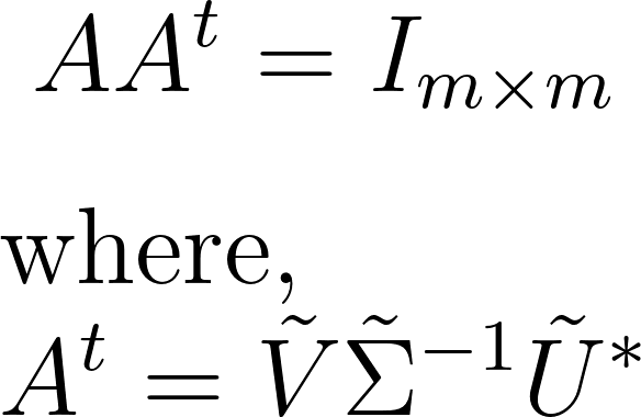
We achieve this using the Moore-Penrose left pseudo-inverse technique. Beginning with the linear problem Ax = b, we substitute the truncated SVD of A. Leveraging the Moore-Penrose left pseudo-inverse identity, we invert each of the U, S, and V matrices to find the pseudo-inverse of A. This process mathematically unfolds as:

Subsequently, we utilize this pseudo-inverse to derive both the minimum-norm and least-squares solutions:

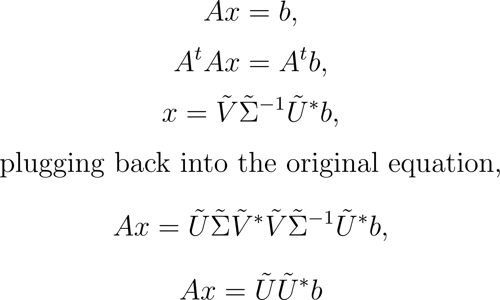
It’s important to note that we utilize the truncated matrix A, not the full SVD matrix, for efficiency. Moreover, UU* represents a projection into the column space of U, indicating that x is the exact solution to Ax = b only when b resides in the column space of U and, consequently, in the column space of A.

Computing the pseudo-inverse of A is computationally efficient post the upfront cost of computing an SVD. Inverting the unitary matrices involves matrix multiplications by transpose, requiring O{nn} operations. Inverting the S matrix is even more efficient due to its diagonal nature, necessitating O{n} operations. Conversely, inverting a dense square matrix would demand O{nn*n} operations, leading to computational challenges. Let’s illustrate this with an examples of linear regression.

Linear regression serves as a vital tool for establishing relationships between variables based on data. Imagine a dataset with a linear relationship characterized by a constant slope. Leveraging the pseudo-inverse, we can determine the least-squares solution for this slope, as demonstrated below:

Understanding this concept is best facilitated through an example. Let’s start by generating a toy dataset. In your Jupyter notebook, ensure you’ve imported the required modules. Utilizing NumPy and Matplotlib, follow these steps to generate and visualize the toy dataset:

### import modules
import numpy as np
import matplotlib.pyplot as plt
from matplotlib import colors
import math as mt
from numpy import linalg as LA

plt.rcParams.update({'font.size' : 22, 'font.family' : 'Times New Roman', "text.usetex": True})

### Toy dataset
x = 3 # True slope
a = np.arange(-2,2,0.25)
a = a.reshape(-1, 1)
b = x*a + np.random.randn(*a.shape) # Add noise

fig, ax = plt.subplots()

ax.scatter(a, b, color = 'k', label = 'Data')
ax.plot(a, a*x, color = 'r', label = 'True Line')

ax.set_xlabel(r'$a$')
ax.set_ylabel(r'$b$')
ax.xaxis.set_tick_params(direction='in', which='both')
ax.yaxis.set_tick_params(direction='in', which='both')
ax.xaxis.set_ticks_position('both')
ax.yaxis.set_ticks_position('both')

ax.legend(loc = 'best', frameon = False) # or 'best', 'upper right', etc

plt.show()

Plotting the dataset will yield the following figure: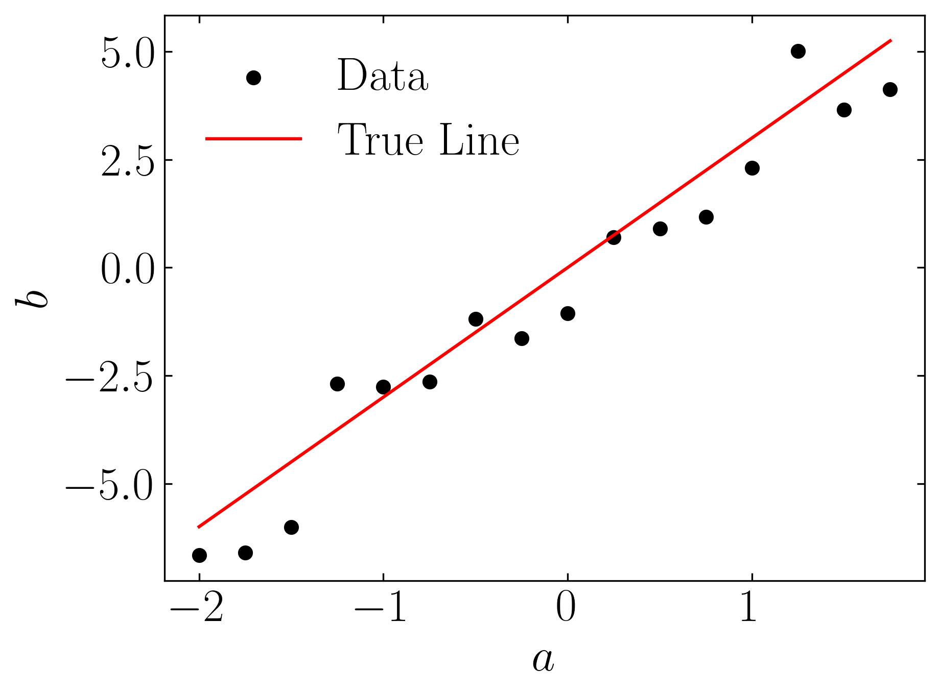

Now, let’s perform the economical SVD of A and use that to generate a least-squares fit for our dataset. This procedure is called linear regression.

U, S, VT = np.linalg.svd(a,full_matrices=False)
xtilde = VT.T @ np.linalg.inv(np.diag(S)) @ U.T @ b # Least-square fit

### Plot 
fig, ax = plt.subplots()

ax.scatter(a, b, color = 'k', label = 'Data')
ax.plot(a, a*x, color = 'r', label = 'True Line')
ax.plot(a, a*xtilde, color = 'b', label = 'Estimated Line')

ax.set_xlabel(r'$a$')
ax.set_ylabel(r'$b$')
ax.xaxis.set_tick_params(direction='in', which='both')
ax.yaxis.set_tick_params(direction='in', which='both')
ax.xaxis.set_ticks_position('both')
ax.yaxis.set_ticks_position('both')

ax.legend(loc = 'best', frameon = False) # or 'best', 'upper right', etc

plt.show()

This procedure yields an approximate solution as shown below: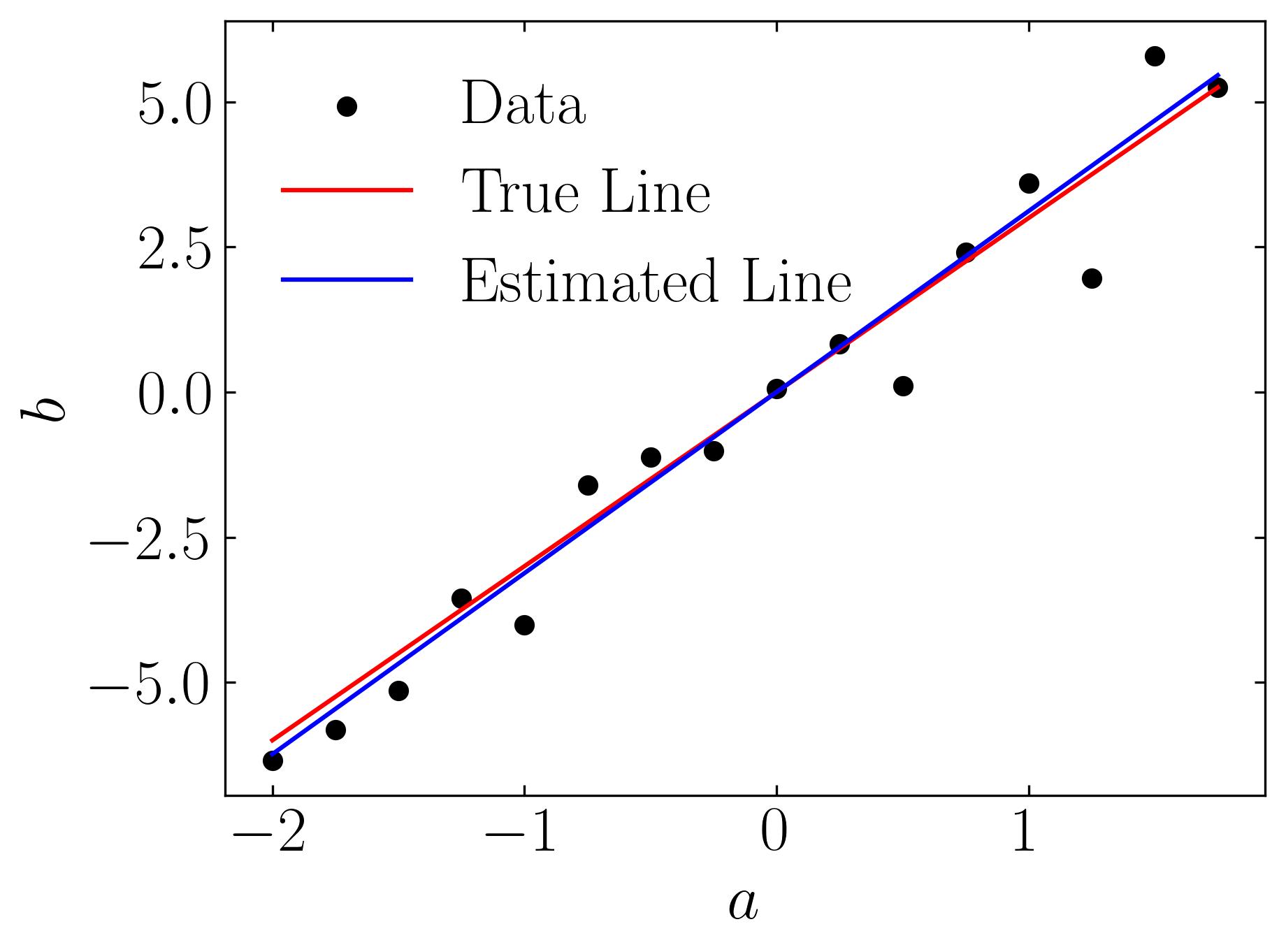

Of course, this whole process has been streamlined using multiple Python packages such as numpy.linalg.lstsq. This is demonstrated in the following example:

x_hat, _, _, _ = LA.lstsq(a[:, np.newaxis], b)

### Plot
fig, ax = plt.subplots()

ax.scatter(a, b, color = 'k', label = 'Data')
ax.plot(a, a*x, color = 'r', label = 'True Line')
ax.plot(a, a*x_hat, color = 'b', label = 'Estimated Line')

ax.set_xlabel(r'$a$')
ax.set_ylabel(r'$b$')
ax.xaxis.set_tick_params(direction='in', which='both')
ax.yaxis.set_tick_params(direction='in', which='both')
ax.xaxis.set_ticks_position('both')
ax.yaxis.set_ticks_position('both')

ax.legend(loc = 'best', frameon = False) # or 'best', 'upper right', etc

plt.show()

Other methods of computing regression include,

xtilde1 = VT.T @ np.linalg.inv(np.diag(S)) @ U.T @ b
xtilde2 = np.linalg.pinv(a) @ b

As we conclude our exploration of Singular Value Decomposition (SVD), we’ve witnessed its transformative power in uncovering hidden patterns and streamlining data analysis workflows. From image compression to linear regression, SVD’s versatility offers a glimpse into the realm of possibilities for extracting insights and making informed decisions. As we continue to delve deeper into the realm of data science, let us harness the potential of SVD to navigate complex datasets and unlock new avenues for exploration and discovery