Eigenfaces, a classic application of Singular Value Decomposition (SVD) and Principal Component Analysis (PCA), revolutionized facial recognition in the realm of computer vision. By representing faces as linear combinations of ‘eigenfaces,’ these techniques offer a powerful method for facial feature extraction, dimensionality reduction, and pattern recognition. PS, one can appreciate the versatility of SVD and PCA across diverse fields, from facial recognition to fluid dynamics, in extracting valuable insights from complex data and enhancing our understanding of underlying structures and patterns.

In the realm of computer vision, the Eigenfaces method stands as a seminal breakthrough, transforming the landscape of facial recognition and pattern analysis. At its core lies a powerful blend of mathematical techniques, specifically Singular Value Decomposition (SVD) and Principal Component Analysis (PCA), which together unravel the complex tapestry of facial images into a concise representation of essential features. One of the pioneering applications of Eigenfaces emerged through the exploration of the Yale Face Database, a treasure trove of facial images capturing variations in lighting, expression, and pose across multiple subjects. By harnessing the computational prowess of SVD and PCA, researchers embarked on a journey to distill the essence of facial characteristics, paving the way for robust identification systems and advancing our understanding of human perception and cognition. In this exploration, we delve into the intricacies of the Eigenfaces problem, tracing its roots in the Yale dataset, and unraveling the transformative impact of SVD and PCA on facial recognition.

However, the influence of SVD and PCA extends far beyond the realm of facial recognition, finding intriguing applications in fluid mechanics. In this interdisciplinary journey, these mathematical tools unveil hidden structures within turbulent flows, offering insights into the dynamics of fluid motion. By applying SVD to velocity fields captured through experimental or computational fluid dynamics (CFD) techniques, researchers can identify coherent flow structures, such as vortices and eddies, amidst the seemingly chaotic turbulence. Moreover, PCA aids in the dimensionality reduction of flow data, enabling the extraction of dominant flow features and simplifying the analysis of complex flow phenomena.

This convergence of computer vision and fluid mechanics highlights the universality of SVD and PCA as indispensable tools for uncovering patterns and extracting essential information from high-dimensional data. Through the lens of Eigenfaces and fluid dynamics, we embark on a journey that transcends disciplinary boundaries, driven by the common quest to decipher the underlying structures shaping our world.

Lets begin!!

EigenFaces

Singular Value Decomposition (SVD) and Principal Component Analysis (PCA) present an array of compelling applications, with one of the most intriguing being the eigenfaces example. In this context, PCA is applied to a vast collection of facial images to discern the most prominent correlations among them, resulting in what are termed as Eigenfaces. These Eigenfaces encapsulate the essence of the image dataset through decomposition. This methodology finds its utility in tasks such as facial recognition and classification within the realms of computer vision and artificial intelligence. Essentially, it serves as an unsupervised dimensionality reduction algorithm (PCA), adept at eliminating non-essential features (dimensions).

The inception of employing eigenfaces for recognition traces back to the pioneering work of Sirovich and Kirby in 1987, with further refinement by Matthew Turk and Alex Pentland around 1991 in the domain of face classification. However, it’s crucial to recognize that this approach, like any other, harbors its own set of advantages and limitations.

Pros: The algorithm boasts simplicity and efficiency, both in terms of computational time and storage requirements. PCA efficiently reduces the dimensionality of facial images, rendering it a highly practical choice for facial recognition tasks.

Cons: Despite its efficacy, the accuracy of the approach diminishes under varying conditions such as fluctuations in light intensity and changes in head positioning. While techniques like head pose estimation coupled with bounding box reorientation can mitigate the latter issue to an extent, the preprocessing entailed to achieve satisfactory results underscores the necessity for continued innovation in the realm of facial recognition algorithms.

Dataset

In this demonstration, we will leverage the Yale Face Database, a comprehensive repository encompassing 38 individuals portrayed in 9 distinct poses under 64 varied lighting conditions. You can access the dataset here. Additionally, for the mathematical underpinnings and conceptual framework, we draw from the seminal work “Data Driven Science and Engineering: Machine Learning, Dynamical Systems and Control” authored by Steven L. Brunton and J. Nathan Kutz.

To embark on this journey, let’s begin by acquiring the dataset. You can download it from this repository.

Furthermore, for a comprehensive understanding of the mathematical methodologies and conceptual paradigms employed, I highly recommend referring to the aforementioned book by Brunton and Kutz.

Now, let’s dive into the practical implementation. Fire up your Jupyter notebook and ensure that you have all the necessary modules loaded. Let’s proceed by importing them:

import numpy as np
import matplotlib.pyplot as plt
from matplotlib import colors
import math as mt
from numpy import linalg as LA
import pandas as pd
import scipy as sp
from time import time
import os
import io

plt.rcParams.update({'font.size' : 22, 'font.family' : 'Times New Roman', "text.usetex": True})

Following the previous steps, ensure you’ve downloaded the allFaces.mat data file from the provided link and placed it within your working directory. Now, within your Jupyter notebook, let’s proceed to load up the data:

mat_contents = sp.io.loadmat('allFaces.mat')
faces = mat_contents['faces']
m = int(mat_contents['m'])
n = int(mat_contents['n'])
nfaces = np.ndarray.flatten(mat_contents['nfaces'])

y = np.zeros((faces.shape[1],)) # Creating labels
j = 0
classes = list(range(len(nfaces)))
for i in nfaces:
  y[j:j+i] = classes.pop(0)
  j = j + i

print("Total dataset size:")
print(f"n_samples: {faces.shape[1]}")
print(f"n_features: {m*n}")
print(f"n_classes: {len(nfaces)}")

Output:

Total dataset size:
n_samples: 2410
n_features: 32256
n_classes: 38

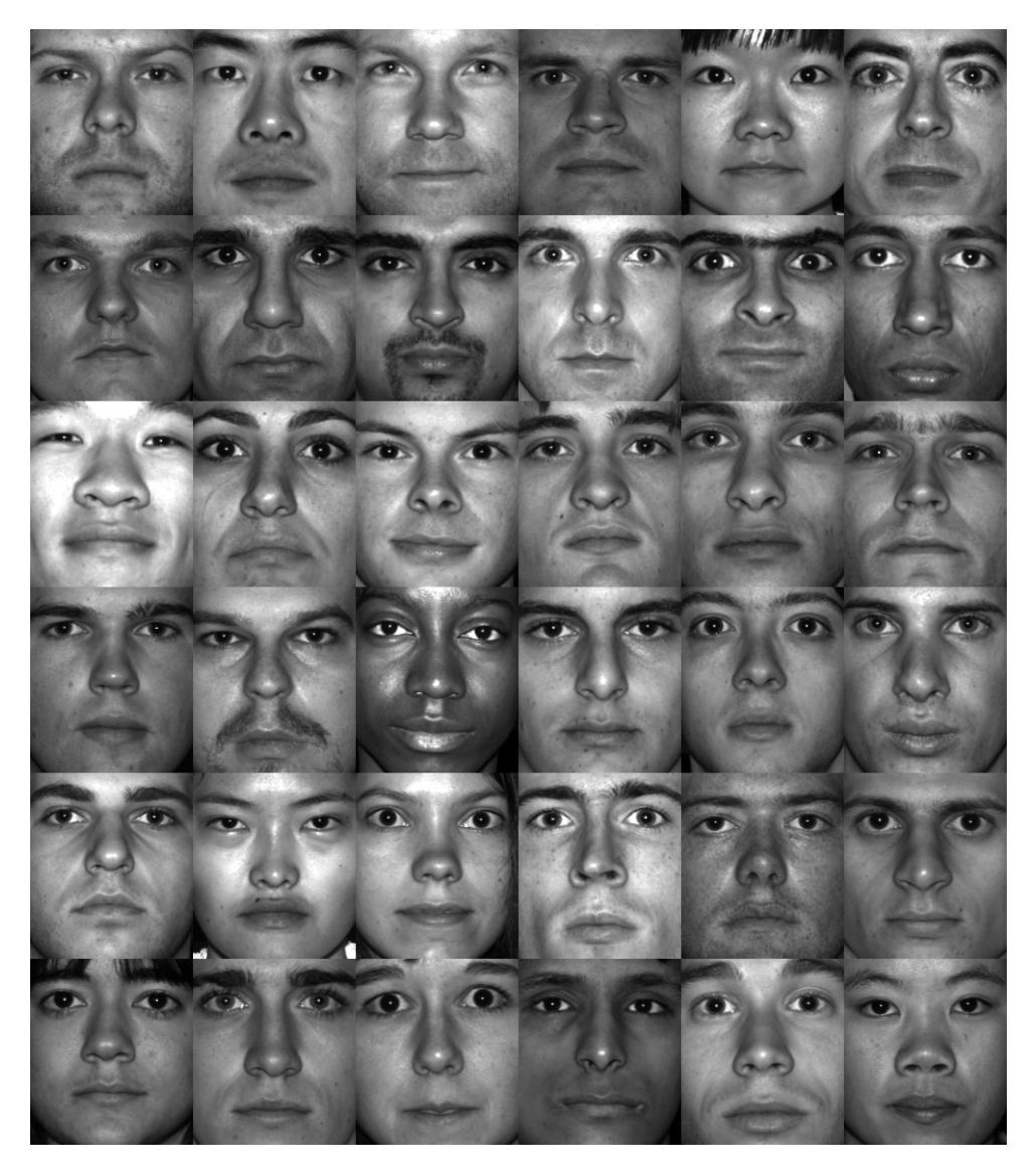
Here, we are considering 38 individual faces (n_classes), each image with 192 x 168 pixels. Each of the facial features in our library are reshaped into a large column array with 192 x 168 = 32256 elements (n_features). Lets visualize an array of images consisting each person from this dataset:

allPersons = np.zeros((n*6,m*6))
count = 0

for j in range(6):
    for k in range(6):
        allPersons[j*n : (j+1)*n, k*m : (k+1)*m] = np.reshape(faces[:,np.sum(nfaces[:count])],(m,n)).T
        count += 1
        
img = plt.imshow(allPersons)
img.set_cmap('gray')
plt.axis('off')

plt.show()

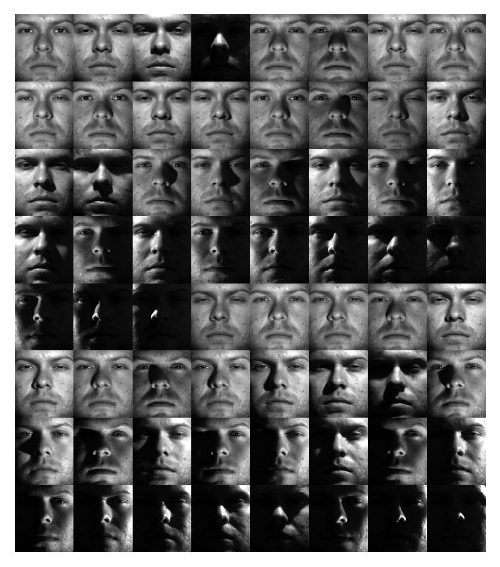
One can also visualize all the poses and lighting conditions by,

Person = 0 # Change the person number here, range(len(nfaces))

subset = faces[:,sum(nfaces[:Person]) : sum(nfaces[:(Person+1)])]
allFaces = np.zeros((n*8,m*8))
    
count = 0
    
for j in range(8):
    for k in range(8):
        if count < nfaces[Person]:
            allFaces[j*n:(j+1)*n,k*m:(k+1)*m] = np.reshape(subset[:,count],(m,n)).T
            count += 1
                
img = plt.imshow(allFaces)
img.set_cmap('gray')
plt.axis('off')
plt.show()

Training

Let’s outline our strategy for leveraging this dataset. Our approach entails utilizing the initial 36 facial images as our training dataset, employing a machine learning algorithm grounded in PCA/SVD principles. Given the total of 38 faces, we reserve the remaining 2 images for validation purposes. Subsequently, we aim to employ this algorithm as a potent tool for both facial recognition and reconstruction tasks, evaluating its efficacy using the reserved test data.

Our journey commences with the acquisition of the first 36 faces from the dataset, followed by the computation of the average facial representation:

# We use the first 36 people for training data
trainingFaces = faces[:,:np.sum(nfaces[:36])]
avgFace = np.mean(trainingFaces,axis=1) # size n*m by 1

Following the data selection and average face computation, the next step involves visualizing both the training faces and the computed average face:

img = plt.imshow(np.reshape(avgFace,(m,n)).T)
img.set_cmap('gray')
plt.axis('off')
plt.show()

Person = 0 # Change the person number here, range(len(nfaces))

img = plt.imshow(np.reshape(trainingFaces[:,np.sum(nfaces[:Person])],(m,n)).T)
img.set_cmap('gray')
plt.axis('off')
plt.show()

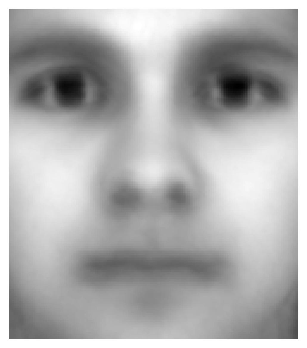
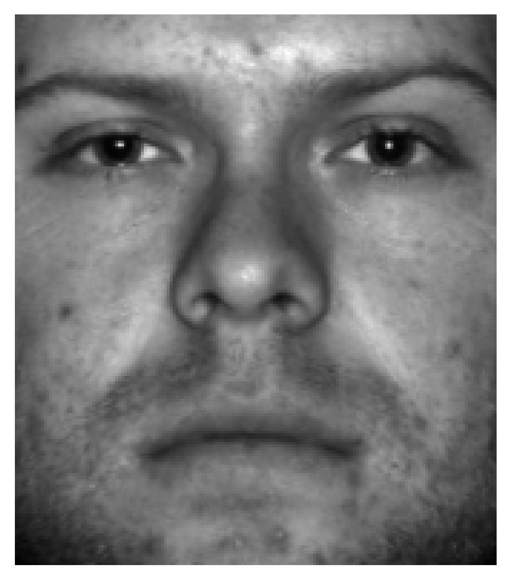
To elucidate the process of assembling the training and average face arrays, let’s visualize the steps undertaken. Initially, we collate all 36 faces from our training dataset into an array termed trainingFaces. Subsequently, we compute the average of this array to derive the aveFace array, encapsulating the collective facial features represented within the training dataset. This visualization offers a clear depiction of the sequence of operations involved in constructing these essential arrays.

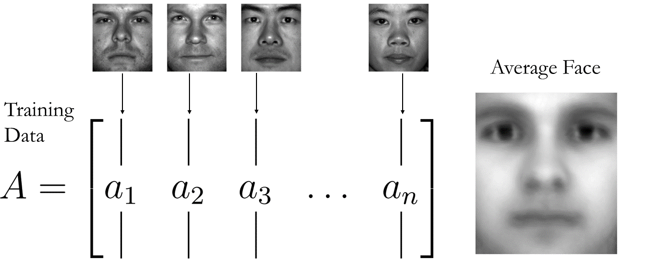
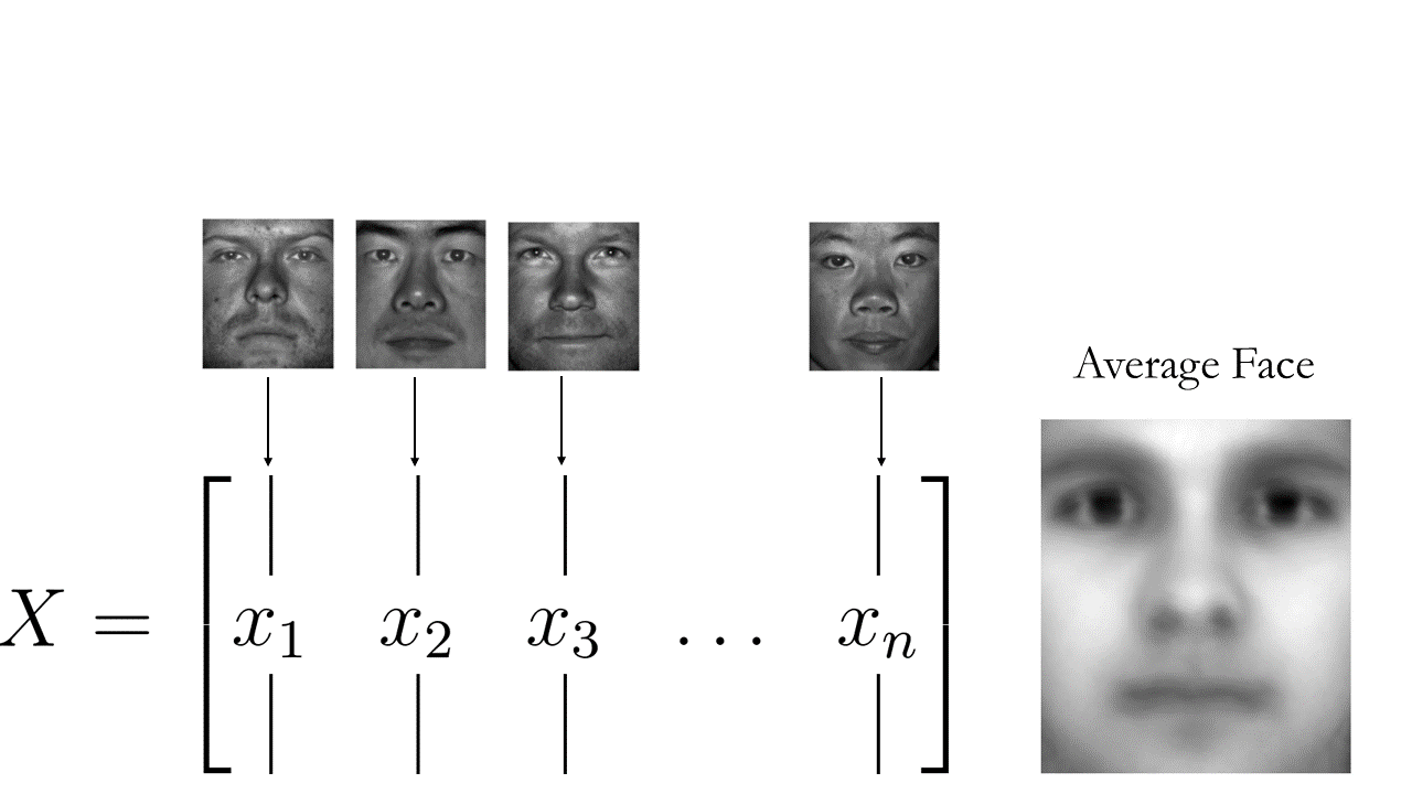
Then simply subtract the average face from the training faces:

X = trainingFaces - np.tile(avgFace,(trainingFaces.shape[1],1)).T

Visualize the mean-subtracted faces:

Person = 0 # Change the person number here, range(len(nfaces))

img = plt.imshow(np.reshape(X[:,np.sum(nfaces[:Person])],(m,n)).T)
img.set_cmap('gray')
plt.axis('off')
plt.show()

Again, our methodology involves subtracting the mean from the training dataset, thereby generating a new matrix termed X, which encompasses the mean-subtracted data. This crucial step facilitates the extraction of essential features while standardizing the dataset for subsequent analysis.

Following the mean subtraction process, our next stride involves computing the Singular Value Decomposition (SVD) of the mean-subtracted faces matrix, effectively culminating in Principal Component Analysis (PCA). This pivotal transformation yields eigenvectors encapsulating the principal components of the dataset, which, when reshaped back to the original 192x168 image grid, manifest as the fundamental components known as eigenfaces. This pivotal procedure enables the extraction and representation of significant facial features, laying the groundwork for subsequent facial recognition and reconstruction endeavors.

# Compute eigenfaces on mean-subtracted training data
print("Computing eigenfaces / Performing SVD on face library")
t0 = time()
U, S, VT = np.linalg.svd(X,full_matrices=0)
print(f"done in {time()-t0:0.3f}s")

To verify the variability inherent within our dataset subsequent to computing the Singular Value Decomposition (SVD), we’ll plot the eigenvalues alongside their cumulative sum, offering insights into the distribution and cumulative contribution of each eigenvalue:

fig, axes = plt.subplots(1, 2, figsize = (10,4))

ax = axes[0]
ax.plot(S, marker = 'o', ls='', markerfacecolor = 'none', markeredgecolor='k')
ax.set_xlabel(r'$r$')
ax.set_ylabel('Singular Values,' + r'$\sigma_n$')
ax.xaxis.set_tick_params(direction='in', which='both')
ax.yaxis.set_tick_params(direction='in', which='both')
ax.xaxis.set_ticks_position('both')
ax.yaxis.set_ticks_position('both')

ax = axes[1]
ax.plot(np.cumsum(S)/np.sum(S), marker = 'o', ls='', markerfacecolor = 'none', markeredgecolor='k')
ax.set_xlabel(r'$r$')
ax.set_ylabel(r'$\sum\sigma_n$')
ax.xaxis.set_tick_params(direction='in', which='both')
ax.yaxis.set_tick_params(direction='in', which='both')
ax.xaxis.set_ticks_position('both')
ax.yaxis.set_ticks_position('both')

plt.tight_layout()

plt.show()

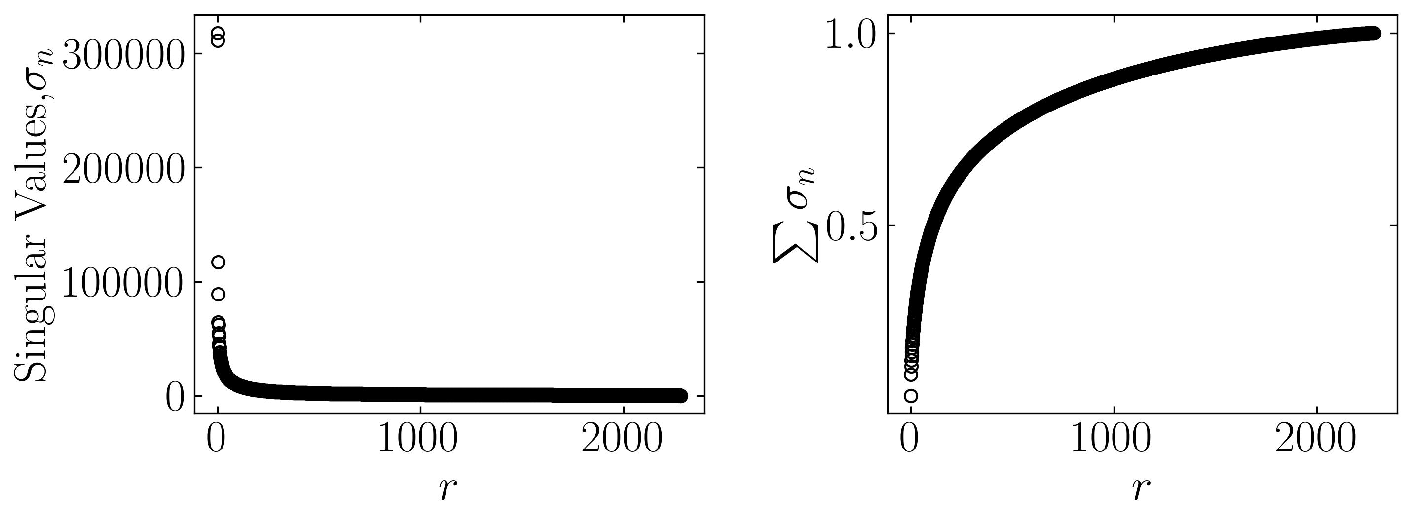
To ascertain the variance score, we can compute it using the cumulative sum of eigenvalues obtained from the Singular Value Decomposition (SVD). This score encapsulates the proportion of variance retained by each principal component. Here’s how you can calculate it:

n_components = [100, 150, 200, 250, 300, 350, 400, 450, 500, 550, 600, 650, 700, 750, 800, 850, 900, 950, 1000]
for i in n_components:
    var = np.sum(S[:i])/np.sum(S)
    print(f"Amount of variance captured by first {i} eigenfaces: {var*100:.1f}")

Output:

Amount of variance captured by first 100 eigenfaces: 48.2
Amount of variance captured by first 150 eigenfaces: 55.1
Amount of variance captured by first 200 eigenfaces: 60.1
Amount of variance captured by first 250 eigenfaces: 64.0
Amount of variance captured by first 300 eigenfaces: 67.2
Amount of variance captured by first 350 eigenfaces: 69.9
Amount of variance captured by first 400 eigenfaces: 72.2
Amount of variance captured by first 450 eigenfaces: 74.3
Amount of variance captured by first 500 eigenfaces: 76.1
Amount of variance captured by first 550 eigenfaces: 77.8
Amount of variance captured by first 600 eigenfaces: 79.3
Amount of variance captured by first 650 eigenfaces: 80.7
Amount of variance captured by first 700 eigenfaces: 82.0
Amount of variance captured by first 750 eigenfaces: 83.2
Amount of variance captured by first 800 eigenfaces: 84.3
Amount of variance captured by first 850 eigenfaces: 85.3
Amount of variance captured by first 900 eigenfaces: 86.3
Amount of variance captured by first 950 eigenfaces: 87.2
Amount of variance captured by first 1000 eigenfaces: 88.1

The variance score plays a pivotal role in guiding the selection of principal components for the facial recognition algorithm. The insights gleaned from these results indicate that a substantial proportion of variance is effectively captured by the initial principal components derived from this dataset. This observation underscores the presence of a pronounced correlation among the distinctive facial features, implying an overlap in the facial characteristics among the 36 individuals represented in our training dataset.

Armed with this understanding, we can confidently proceed with testing our trained model on the two faces reserved for validation, leveraging the insights garnered from the PCA analysis to inform our subsequent facial recognition endeavors. This strategic approach ensures the efficacy and generalizability of our model across diverse facial representations.

Testing the Algorithm

To evaluate the performance of our facial recognition algorithm, let’s endeavor to approximate one of the test images. We reserved two images at the outset (Person 37 and 38), with Person 37 designated for this evaluation. We will assess how effectively a rank-r Singular Value Decomposition (SVD) basis can approximate this test image. Leveraging the left-singular matrix 𝑈 obtained from the previous SVD, and denoting the test image as 𝑥_test, we can employ the following projection:

This projection enables us to approximate the test image 𝑥_test using a rank-r SVD basis, thereby facilitating the evaluation of our facial recognition algorithm’s performance.

To approximate the eigenface using multiple ranks:

testFace = faces[:,np.sum(nfaces[:37])] # First face of person 37

testFaceMS = testFace - avgFace
r_list = [25, 50, 100, 200, 400, 800, 1600]
width = 4
height = int(np.ceil(len(r_list)/width))
fig4 = plt.figure(figsize=(12, 8))
ax = fig4.add_subplot(height, width, 1)
img = ax.imshow(np.reshape(testFace,(m,n)).T)
img.set_cmap('gray')
ax.set_title('Original Image')
plt.axis('off')

for r in r_list:
    reconFace = avgFace + U[:,:r] @ (U[:,:r].T @ testFaceMS)
    ax = fig4.add_subplot(height, width, r_list.index(r)+2)
    img = ax.imshow(np.reshape(reconFace,(m,n)).T)
    img.set_cmap('gray')
    ax.set_title('r = ' + str(r))
    plt.axis('off')

plt.show()

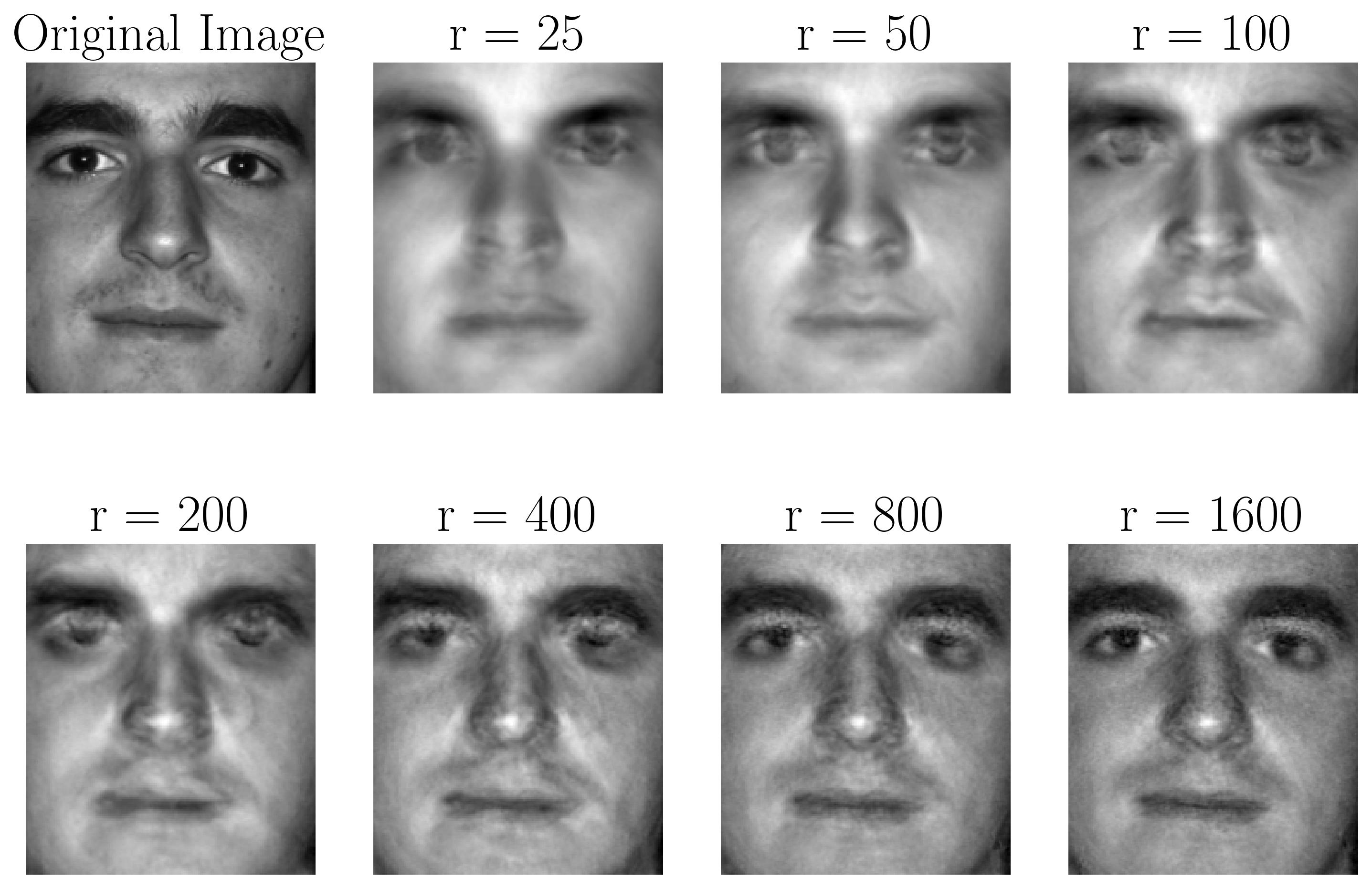
The approximation results indicate suboptimal performance for 𝑟 ≤ 200, suggesting insufficient representation of the test image. However, as the rank-𝑟 surpasses 400, the approximation gradually converges, effectively capturing the essence of the test image. Referring back to the variability score derived earlier, it’s evident that at 𝑟>400, the approximation achieves a representation accuracy exceeding 72%.

This implies that with a rank 400 SVD, our facial recognition algorithm can reconstruct the test image with an accuracy exceeding 72%. Considering the complexity of facial features and the inherent variability across individuals, achieving such a level of accuracy underscores the effectiveness of our algorithm. It’s indeed a commendable outcome, signaling promising prospects for practical deployment and real-world applications.

Testing our algorithm with a distinct face outside the realms of both the test and training datasets offers a compelling validation of its robustness and generalizability. For this evaluation, I’ve selected an image of Dr. Richard Feynman (needs no introduction!!).

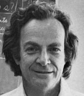
By subjecting Dr. Feynman’s image to our facial recognition algorithm, we can assess its ability to accurately reconstruct and identify a facial representation that deviates significantly from the dataset. This test not only validates the algorithm’s performance in handling novel inputs but also highlights its potential utility in real-world scenarios characterized by diverse facial representations.

### Loading the image
mat = plt.imread('Richard_Feynman.png')
print(mat.T.shape)

fig, ax = plt.subplots()
p = ax.imshow(mat, cmap = 'gray')
plt.show()

### Facial reconstruction algorithm

testFace = np.reshape(mat.T, (m*n)) # New Face

testFaceMS = testFace - avgFace
r_list = [200, 400, 800, 1600, 2000, 2200, 2500]
width = 4
height = int(np.ceil(len(r_list)/width))
fig4 = plt.figure(figsize=(12, 8))
ax = fig4.add_subplot(height, width, 1)
img = ax.imshow(np.reshape(testFace,(m,n)).T)
img.set_cmap('gray')
ax.set_title('Original Image')
plt.axis('off')

for r in r_list:
    reconFace = avgFace + U[:,:r] @ (U[:,:r].T @ testFaceMS)
    ax = fig4.add_subplot(height, width, r_list.index(r)+2)
    img = ax.imshow(np.reshape(reconFace,(m,n)).T)
    img.set_cmap('gray')
    ax.set_title('r = ' + str(r))
    plt.axis('off')

plt.show()

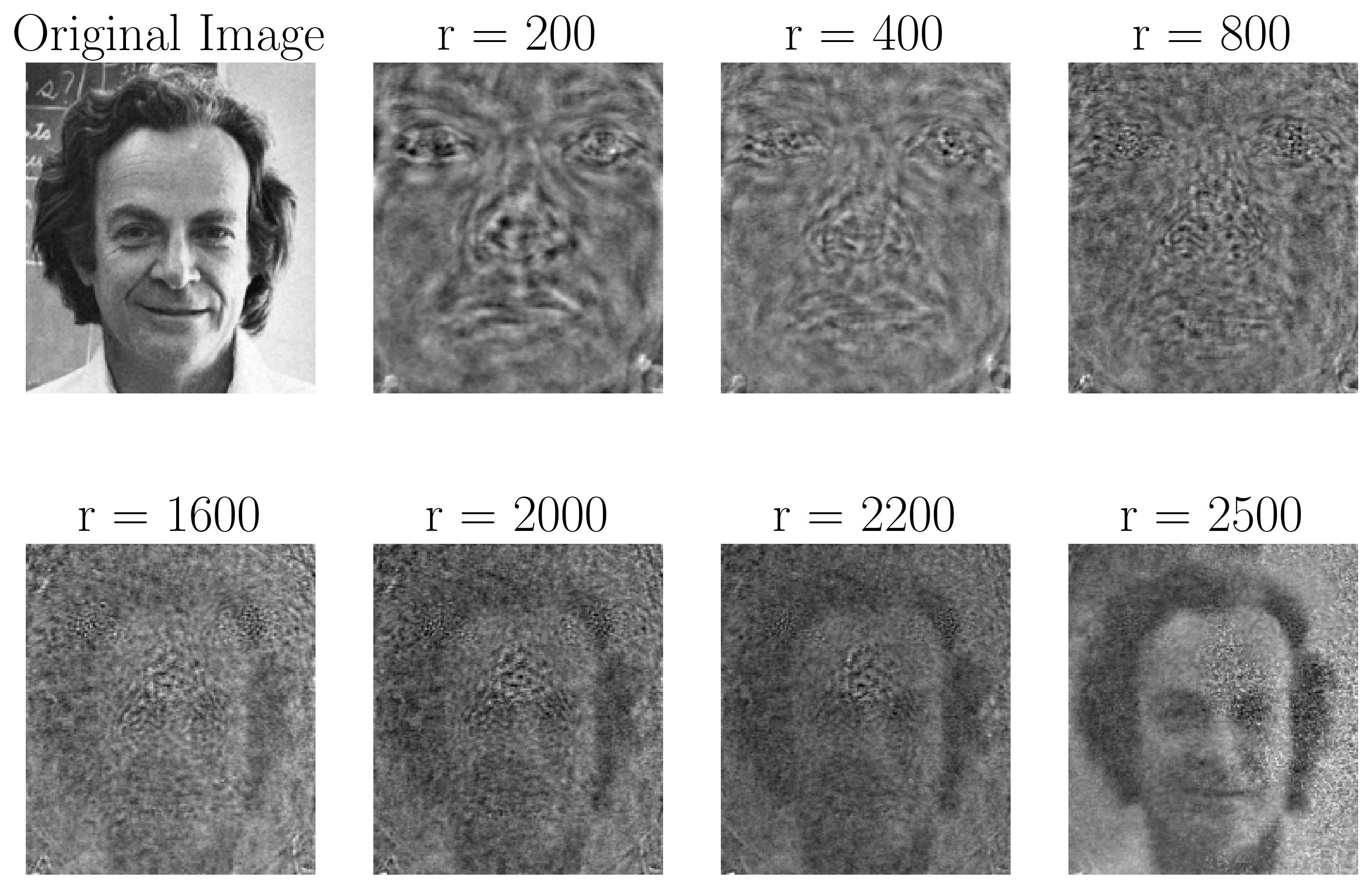
Indeed, the eigenfaces space possesses a remarkable capability to approximate images, even those of individuals not included in the training dataset, such as Dr. Feynman. This phenomenon is attributable to the expansive nature of the eigenfaces space, which spans a substantial subspace within the 32256-dimensional image (192 x 168) space. The eigenfaces collectively encapsulate broad, smooth, and non-localized spatial features intrinsic to facial structures, including cheeks, forehead, mouths, and other facial attributes. Consequently, even in the absence of specific training data for Dr. Feynman, the algorithm leverages these foundational facial components to effectively reconstruct and approximate his image. This underscores the versatility and adaptability of the eigenfaces approach, rendering it a potent tool for facial recognition and reconstruction tasks across diverse datasets and individuals.

PCA’s efficacy in discerning discriminant features crucial for facial recognition is noteworthy. Up to this juncture, our analysis has predominantly focused on a single pose and optimal lighting conditions within the training dataset. However, it’s imperative to extend our investigation to encompass the broader spectrum of variations, including different poses and lighting conditions. By harnessing PCA, we can effectively classify these diverse features, commencing with an exploration of the lighting conditions. Utilizing the eigenfaces as a coordinate system, we delineate an eigenface space, wherein each eigenface serves as a basis vector. This enables the projection of an image 𝑥 into the first 𝑟 PCA modes, yielding a set of coordinates within this space:

The resulting eigenface space encapsulates a rich array of features. Certain principal components capture ubiquitous facial attributes shared across individuals, while others discern unique characteristics distinguishing one individual from another. Furthermore, additional principal components adeptly capture the nuances of lighting effects, thereby enhancing the algorithm’s capacity to discriminate between facial representations under varied lighting conditions. In essence, PCA empowers us to extract and leverage discriminant features essential for effective facial recognition, even amidst the complexities introduced by diverse poses and lighting conditions.

P1num = 2 # Person number 2
P2num = 7 # Person number 7

P1 = faces[:, np.sum(nfaces[:(P1num-1)]):np.sum(nfaces[:P1num])]
P2 = faces[:, np.sum(nfaces[:(P2num-1)]):np.sum(nfaces[:P2num])]

P1 = P1 - np.tile(avgFace, (P1.shape[1],1)).T
P2 = P2 - np.tile(avgFace, (P2.shape[1],1)).T

PCAmodes = [5, 6]
PCACoordsP1 = U[:, PCAmodes-np.ones_like(PCAmodes)].T @ P1
PCACoordsP2 = U[:, PCAmodes-np.ones_like(PCAmodes)].T @ P2

fig, ax = plt.subplots()
ax.plot(PCACoordsP1[0, :], PCACoordsP1[1, :], 'd', color='k', label=f"Person {P1num}")
ax.plot(PCACoordsP2[0, :], PCACoordsP2[1, :], '^', color='r', label=f"Person {P2num}")

ax.plot(PCACoordsP1[0, 2], PCACoordsP1[1, 2], marker = 'd', ls='', markerfacecolor = 'none', 
        markeredgewidth=2, markeredgecolor='g', label=f"Person {P1num}")
ax.plot(PCACoordsP2[0, 2], PCACoordsP2[1, 2], marker = '^', ls='', markerfacecolor = 'none', 
        markeredgewidth=2, markeredgecolor='g', label=f"Person {P2num}")

ax.plot(PCACoordsP1[0, 3], PCACoordsP1[1, 3], marker = 'd', ls='', markerfacecolor = 'none', 
        markeredgewidth=2, markeredgecolor='g', label=f"Person {P1num}")
ax.plot(PCACoordsP2[0, 3], PCACoordsP2[1, 3], marker = '^', ls='', markerfacecolor = 'none', 
        markeredgewidth=2, markeredgecolor='g', label=f"Person {P2num}")

ax.plot(PCACoordsP1[0, 4], PCACoordsP1[1, 4], marker = 'd', ls='', markerfacecolor = 'none', 
        markeredgewidth=2, markeredgecolor='g', label=f"Person {P1num}")
ax.plot(PCACoordsP2[0, 4], PCACoordsP2[1, 4], marker = '^', ls='', markerfacecolor = 'none', 
        markeredgewidth=2, markeredgecolor='g', label=f"Person {P2num}")

ax.set(xlabel="PC 5", ylabel="PC 6")
ax.set_xticks([0])
ax.set_yticks([0])

plt.grid()
plt.show()

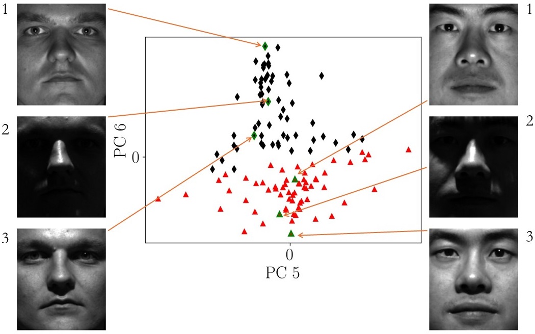
The visualization above showcases the coordinates of all 64 images (representing various lighting conditions) of two individuals projected into the 5th and 6th principal components derived from the eigenface space. Notably, the images of the two individual faces exhibit discernible separation in these coordinates. This observation underscores PCA’s efficacy in extracting discriminant features capable of distinguishing between distinct individuals, even amidst the myriad variations introduced by different lighting conditions.

This compelling demonstration underscores PCA’s potential to serve as the cornerstone of an image recognition and classification algorithm. By leveraging the rich feature representation provided by PCA, we can effectively discern subtle nuances and variations within facial images, facilitating accurate classification and recognition tasks across diverse datasets and conditions. This highlights PCA’s versatility and utility as a powerful tool in the realm of image processing and pattern recognition.