Demystify Fluid Flow with Dynamic Mode Decomposition (DMD)
Fluid flows, with their mesmerizing swirls and eddies, are prime examples of complex systems. But hidden within this complexity lies order! This blog post delves into how Dynamic Mode Decomposition (DMD) can be applied to unlock the secrets of fluid flow data. We’ll explore how DMD extracts meaningful patterns, providing valuable insights for scientists and engineers.
Dynamic Mode Decomposition (DMD), pioneered by Schmid (2010) in the fluid dynamics community, revolutionized the identification of spatio-temporal coherent structures from high-dimensional data. Building upon the foundation of Proper Orthogonal Decomposition (POD), DMD leverages the computationally efficient Singular Value Decomposition (SVD), enabling scalable and effective dimensionality reduction in complex systems. Unlike SVD/POD, which prioritizes spatial correlation and energy content, often neglecting temporal dynamics, DMD offers a modal decomposition approach. Here, each mode encapsulates spatially correlated structures exhibiting identical linear behavior over time, such as oscillations at a specific frequency with either growth or decay. Thus, DMD not only streamlines dimensionality reduction by yielding a reduced set of modes but also furnishes a temporal model delineating the evolution of these modes.
In this article, I’ll be showcasing the application of DMD on a dataset portraying a time series of fluid vorticity fields depicting the wake behind a circular cylinder at Reynolds number Re = 100, sourced from Data-Driven Modeling of Complex Systems. To get started, you can download the dataset from this link. Choosing Re = 100 serves as an optimal benchmark due to its significance beyond the critical Reynolds number 47. At this threshold, the flow undergoes a supercritical Hopf bifurcation, resulting in laminar vortex shedding.
Within our computational framework, the domain encompasses 450 × 200 grid points. Employing a time step of Δt = 0.02 ensures compliance with the CFL condition. The simulation harnesses the two-dimensional Navier–Stokes equations, executed through an immersed boundary projection method (IBPM) fluid solver, founded on the fast multidomain method. Snapshots capturing the cylinder wake are gathered post simulations, converging to a state of steady-state vortex shedding. A total of 150 snapshots were meticulously collected at regular intervals of 10Δt, effectively sampling five periods of vortex shedding.
Let’s dive in!
Initial setup
To begin, fire up a Jupyter notebook and import the essential modules:
import matplotlib.colors
import matplotlib.pyplot as plt
import numpy as np
import pandas as pd
import fluidfoam as fl
import scipy as sp
import os
import matplotlib.animation as animation
import pyvista as pv
import imageio
import io
%matplotlib inline
plt.rcParams.update({'font.size' : 20, 'font.family' : 'Times New Roman', "text.usetex": True})
Next, after downloading the dataset as directed earlier, ensure it’s placed in your working directory. Then, in Python, set the path variables by:
Path = 'E:/Blog_Posts/BruntonCylinder/' ### Path to your working folder
save_path = 'E:/Blog_Posts/OpenFOAM/ROM_Series/Post28/' ### Path to your working folder
Files = os.listdir(Path)
print(Files)

### OUTPUT
### ['CYLINDER_ALL.mat', 'CYLINDER_basis.mat', 'VORTALL.mat']
Load the CYLINDER_ALL.mat:
Contents = sp.io.loadmat(Path + Files[0])
Given that this file essentially acts as a dictionary, you can list out its keys using the keys() method:
Contents.keys()

### Output:
### dict_keys(['__header__', '__version__', '__globals__', 'UALL', 'UEXTRA', 'VALL', 'VEXTRA', 'VORTALL', 'VORTEXTRA', 'm', 'n', 'nx', 'ny'])
Let’s begin by extracting the necessary data from this dictionary. This step involves identifying and retrieving the specific information or variables needed for our analysis.
m = Contents['m'][0][0]
n = Contents['n'][0][0]
Vort = Contents['VORTALL']
print(m, n)
print(Vort.shape)

### Output:
### 199 449
### (89351, 151)
Based on this information, we understand that the data comprises 199 x 499 (= 89,351) spatial degrees of freedom and includes 151 available snapshots.
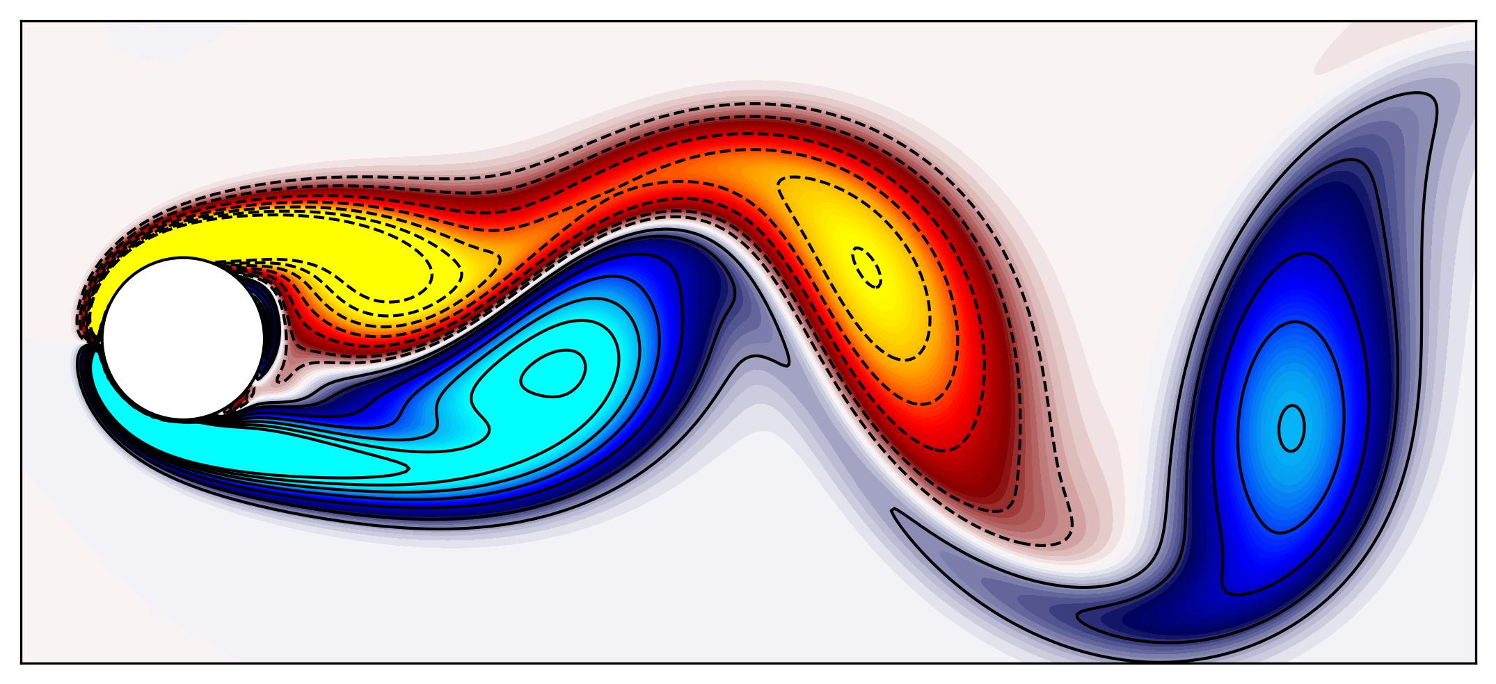
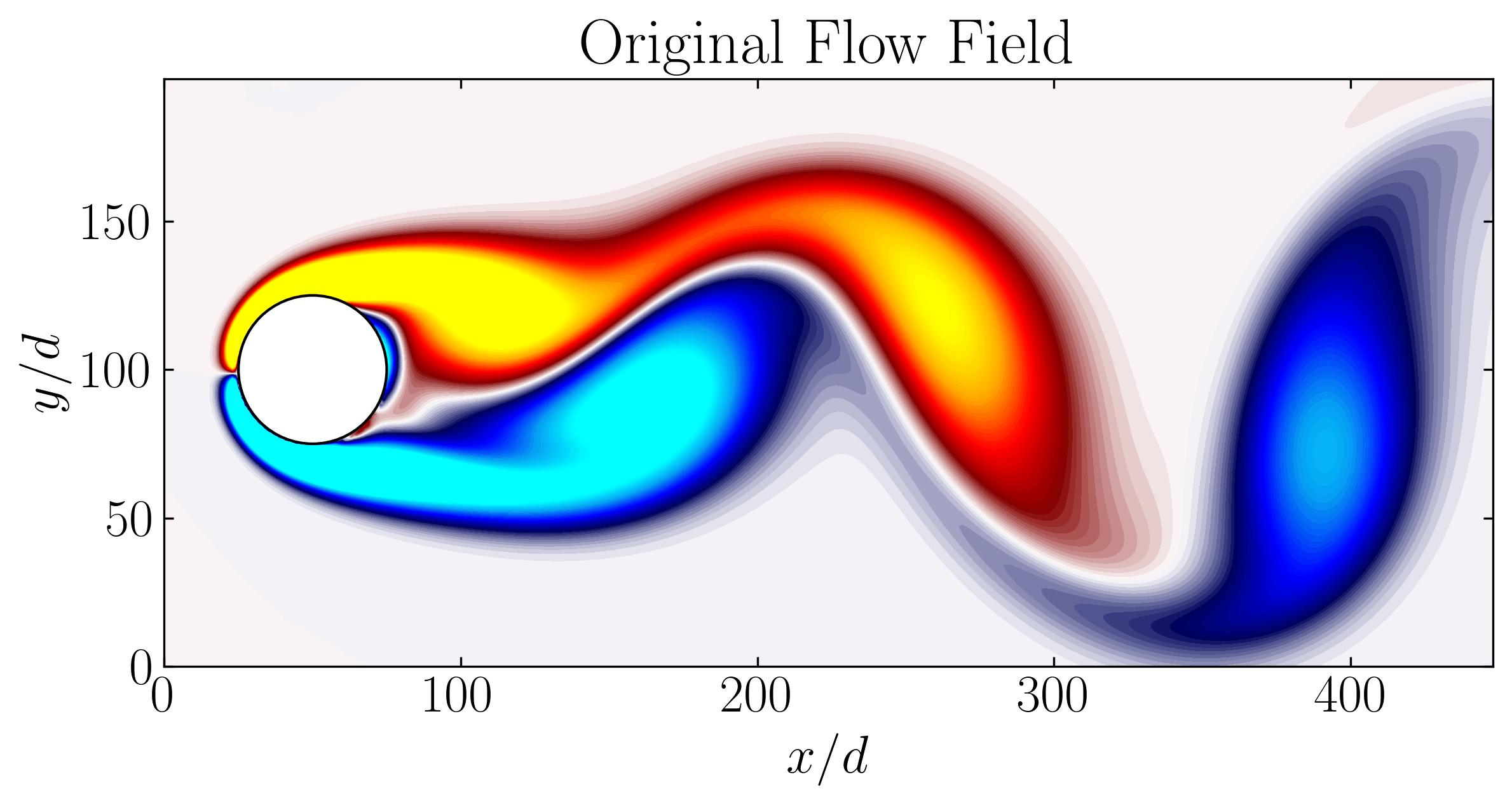
Lets visualize one snapshots using a simple plotting routine in matplotlib:
Circle = plt.Circle((50, 100), 25, ec='k', color='white', zorder=2)

fig, ax = plt.subplots(figsize=(11, 4))
p = ax.contourf(np.reshape(Vort[:,0],(n,m)).T, levels = 1001, vmin=-2, vmax=2, cmap = cmap.reversed())
q = ax.contour(np.reshape(Vort[:,0],(n,m)).T,
               levels = [-2.4, -2, -1.6, -1.2, -0.8, -0.4, -0.2, 0.2, 0.4, 0.8, 1.2, 1.6, 2, 2.4],
               colors='k', linewidths=1)
ax.add_patch(Circle)
ax.set_aspect('equal')
xax = ax.axes.get_xaxis()
xax = xax.set_visible(False)
yax = ax.axes.get_yaxis()
yax = yax.set_visible(False)
plt.show()
Proper Orthogonal Decomposition
Before getting to Dynamic Mode Decomposition, let’s first compute Proper Orthogonal Decomposition (POD) of the flow field. This will aid in determining the appropriate r-rank approximation needed for DMD. As a quick recap, the DMD algorithm relies on Singular Value Decomposition (SVD) reduction to execute a low-rank truncation of the data. If the data harbors low-dimensional structures, the singular values of Σ will sharply decline towards zero, potentially with only a handful of dominant modes.
It’s worth noting that POD can be applied to either fluid velocity field or vorticity field data. In our case, we’ll be utilizing vorticity fields.
Here’s a rundown of the steps for POD:
### POD Analysis

### Data Matrix
X = Vort

### Mean-removed Matrix
X_mean = np.mean(X, axis = 1)
Y = X - X_mean[:,np.newaxis]

### Covariance Matrix
C = np.dot(Y.T, Y)/(Y.shape[1]-1)

### SVD of Covariance Matrix
U, S, V = np.linalg.svd(C)

### POD modes
Phi = np.dot(Y, U)

### Temporal coefficients
a = np.dot(Phi.T, Y)
Now, since the objective behind conducting POD was to ascertain the minimum rank necessary for DMD, let’s visualize the energy content of the POD modes along with the cumulative energy:
Energy = np.zeros((len(S),1))
for i in np.arange(0,len(S)):
    Energy[i] = S[i]/np.sum(S)

X_Axis = np.arange(Energy.shape[0])
heights = Energy[:,0]

fig, axes = plt.subplots(1, 2, figsize = (12,4))
ax = axes[0]
ax.plot(Energy, marker = 'o', markerfacecolor = 'none', markeredgecolor = 'k', ls='-', color = 'k')
ax.set_xlim(0, 20)
ax.set_xlabel('Modes')
ax.set_ylabel('Energy Content')

ax = axes[1]
cumulative = np.cumsum(S)/np.sum(S)
ax.plot(cumulative, marker = 'o', markerfacecolor = 'none', markeredgecolor = 'k', ls='-', color = 'k')
ax.set_xlabel('Modes')
ax.set_ylabel('Cumulative Energy')
ax.set_xlim(0, 20)

plt.show()
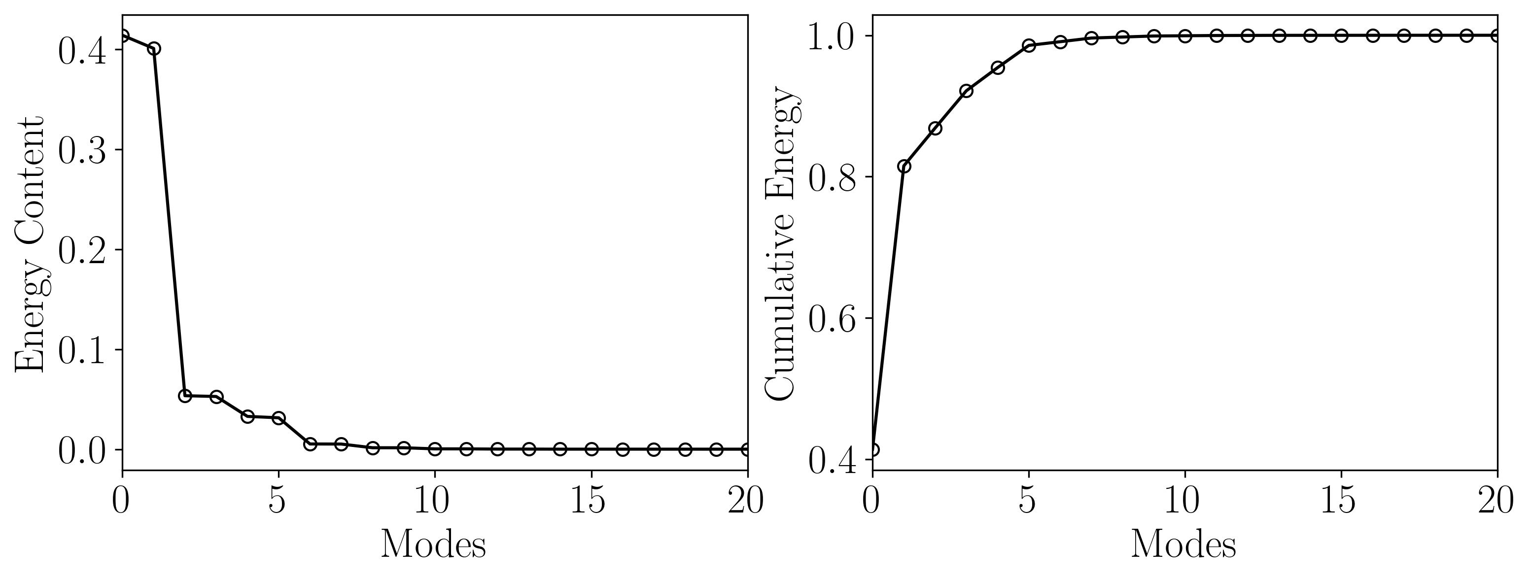
This illustration demonstrates that the initial 10 POD modes encapsulate approximately 97% of the total energy, while the first 21 modes encompass nearly 99.9% of it. Consequently, a rank-21 approximated DMD should effectively capture the predominant dynamics of the flow.
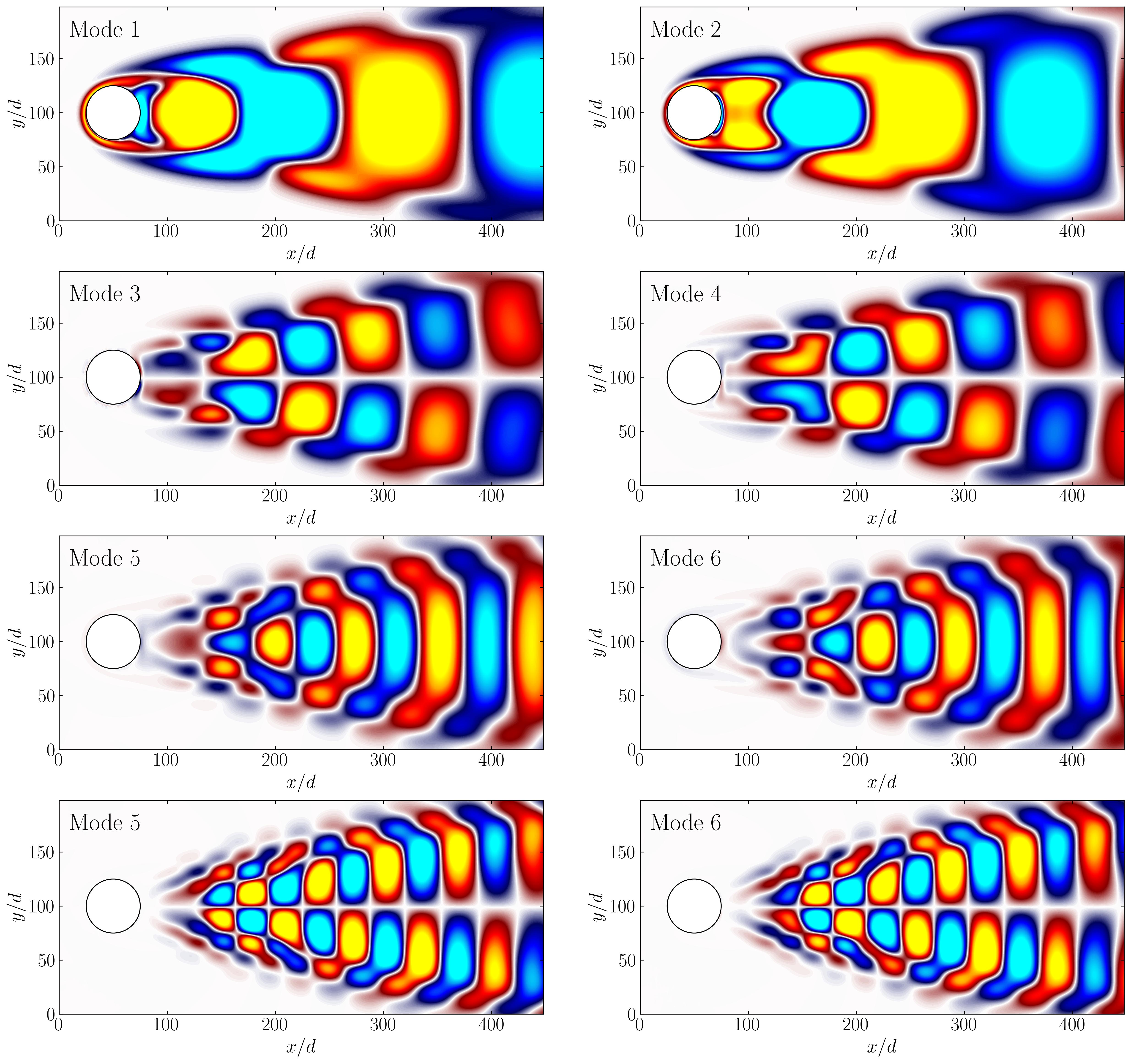
To wrap up, here are the first 8 POD modes for comprehensive reference.
Dynamic Mode Decomposition
Implementing DMD on the cylinder wake necessitates the same fundamental snapshot information as POD, rendering it a data-driven method that seamlessly adapts to data sourced from simulations or experiments.
In this section, we will employ the DMD function from my previous article to compute the DMD modes.
def DMD(X1, X2, r, dt):
    U, s, Vh = np.linalg.svd(X1, full_matrices=False)
    ### Truncate the SVD matrices
    Ur = U[:, :r]
    Sr = np.diag(s[:r])
    Vr = Vh.conj().T[:, :r]

    ### Build the Atilde and find the eigenvalues and eigenvectors
    Atilde = Ur.conj().T @ X2 @ Vr @ np.linalg.inv(Sr)
    Lambda, W = np.linalg.eig(Atilde)

    ### Compute the DMD modes
    Phi = X2 @ Vr @ np.linalg.inv(Sr) @ W

    omega = np.log(Lambda)/dt ### continuous time eigenvalues

    ### Compute the amplitudes

    alpha1 = np.linalg.lstsq(Phi, X1[:, 0], rcond=None)[0] ### DMD mode amplitudes

    b = np.linalg.lstsq(Phi, X2[:, 0], rcond=None)[0] ### DMD mode amplitudes

    ### DMD reconstruction
    time_dynamics = None
    for i in range(X1.shape[1]):
        v = np.array(alpha1)[:,0]*np.exp( np.array(omega)*(i+1)*dt)
        if time_dynamics is None:
            time_dynamics = v
        else:
            time_dynamics = np.vstack((time_dynamics, v))
    X_dmd = np.dot( np.array(Phi), time_dynamics.T)

    return Phi, omega, Lambda, alpha1, b, X_dmd
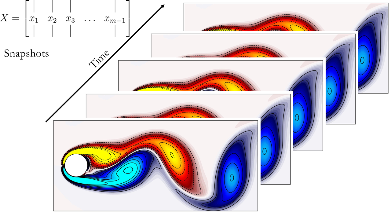
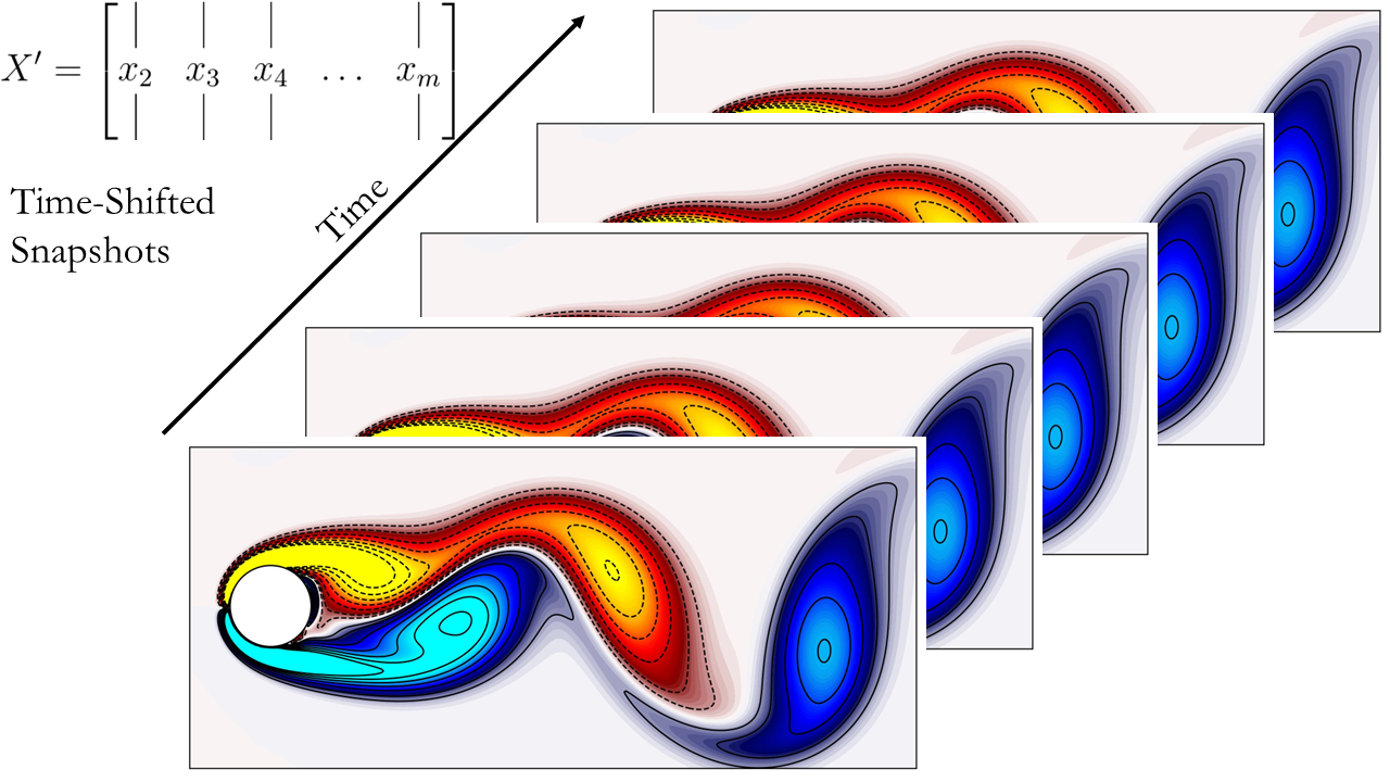
Next, generate the two time-shifted data matrices. For reference, here’s a schematic illustrating the data matrices and their respective representations.
### get two views of the data matrix offset by one time step
X1 = np.matrix(X[:, 0:-1])
X2 = np.matrix(X[:, 1:])

### Constants
r = 21
dt = 0.02*10
Here are the schematics of the data matrices:
Now, let’s proceed to compute DMD.
Phi, omega, Lambda, alpha1, b, X_dmd = DMD(X1, X2, r, dt)
Now that we’ve computed DMD, the next question arises: how should one commence analyzing the DMD data? Let’s start by examining the individual terms we’ve extracted, gathering insights into their size, type, and structure.
print('PhiShape = ', Phi.shape)
print('OmegaShape = ', omega.shape)
print('LambdaShape = ', Lambda.shape)
print('Alpha1Shape = ', alpha1.shape)
print('bShape = ', b.shape)
print('X_dmdShape = ', X_dmd.shape)

print('typePhi = ', Phi.dtype)
print('typeOmega = ', omega.dtype)
print('typeLambda = ', Lambda.dtype)
print('typeAlpha1 = ', alpha1.dtype)
print('typeb = ', b.dtype)
print('typeX_dmd = ', X_dmd.dtype)
Output:
PhiShape =  (89351, 21)
OmegaShape =  (21,)
LambdaShape =  (21,)
Alpha1Shape =  (21, 1)
bShape =  (21, 1)
X_dmdShape =  (89351, 150)
typePhi =  complex128
typeOmega =  complex128
typeLambda =  complex128
typeAlpha1 =  complex128
typeb =  complex128
typeX_dmd =  complex128
Let’s decipher this step by step. Firstly, the shapes of Phi, Omega, Lambda, and alpha reflect the rank-21 approximation, hinting that we’re focusing solely on the most dominant structures in the flow. Additionally, the data type of the different arrays is complex. With this in mind, let’s examine the Lambda array, which represents the eigenvalues.
print(Lambda)
Output:
[-0.48625223+0.87378727j -0.48625223-0.87378727j -0.29541768+0.95537656j
 -0.29541768-0.95537656j -0.09183219+0.99576056j -0.09183219-0.99576056j
  0.11562445+0.99328608j  0.11562445-0.99328608j  1.        +0.j
  0.97847826+0.20635002j  0.97847826-0.20635002j  0.91483931+0.4038178j
  0.91483931-0.4038178j   0.81182274+0.58390345j  0.81182274-0.58390345j
  0.67386251+0.73885682j  0.67386251-0.73885682j  0.31811343+0.9480558j
  0.31811343-0.9480558j   0.50689689+0.86200961j  0.50689689-0.86200961j]
Here, the eigenvalues form a set of complex numbers, each carrying specific significance. Each eigenvalue elucidates the dynamic behavior of its corresponding mode in the following manner:
- If the eigenvalue possesses a non-zero imaginary part, it indicates oscillation in the corresponding dynamic mode.
- If the eigenvalue resides inside the unit circle, the dynamic mode is characterized by decay.
- If the eigenvalue lies outside the unit circle, the dynamic mode exhibits growth.
- If the eigenvalue precisely falls on the unit circle, the mode neither grows nor decays.
Armed with this insight, one can construct a simple unit circle plot and overlay the scatter plot of the real versus imaginary eigenvalues onto it, as demonstrated below:
theta = np.linspace( 0 , 2 * np.pi , 150 )
radius = 1
a = radius * np.cos( theta )
b = radius * np.sin( theta )

fig, ax = plt.subplots()

ax.scatter(np.real(Lambda), np.imag(Lambda), color = 'r', marker = 'o', s = 100)
ax.plot(a, b, color = 'k', ls = '--')

ax.set_xlabel(r'$\Lambda_r$')
ax.set_ylabel(r'$\Lambda_i$')

ax.set_aspect('equal')

plt.show()
This should yield the following plot:
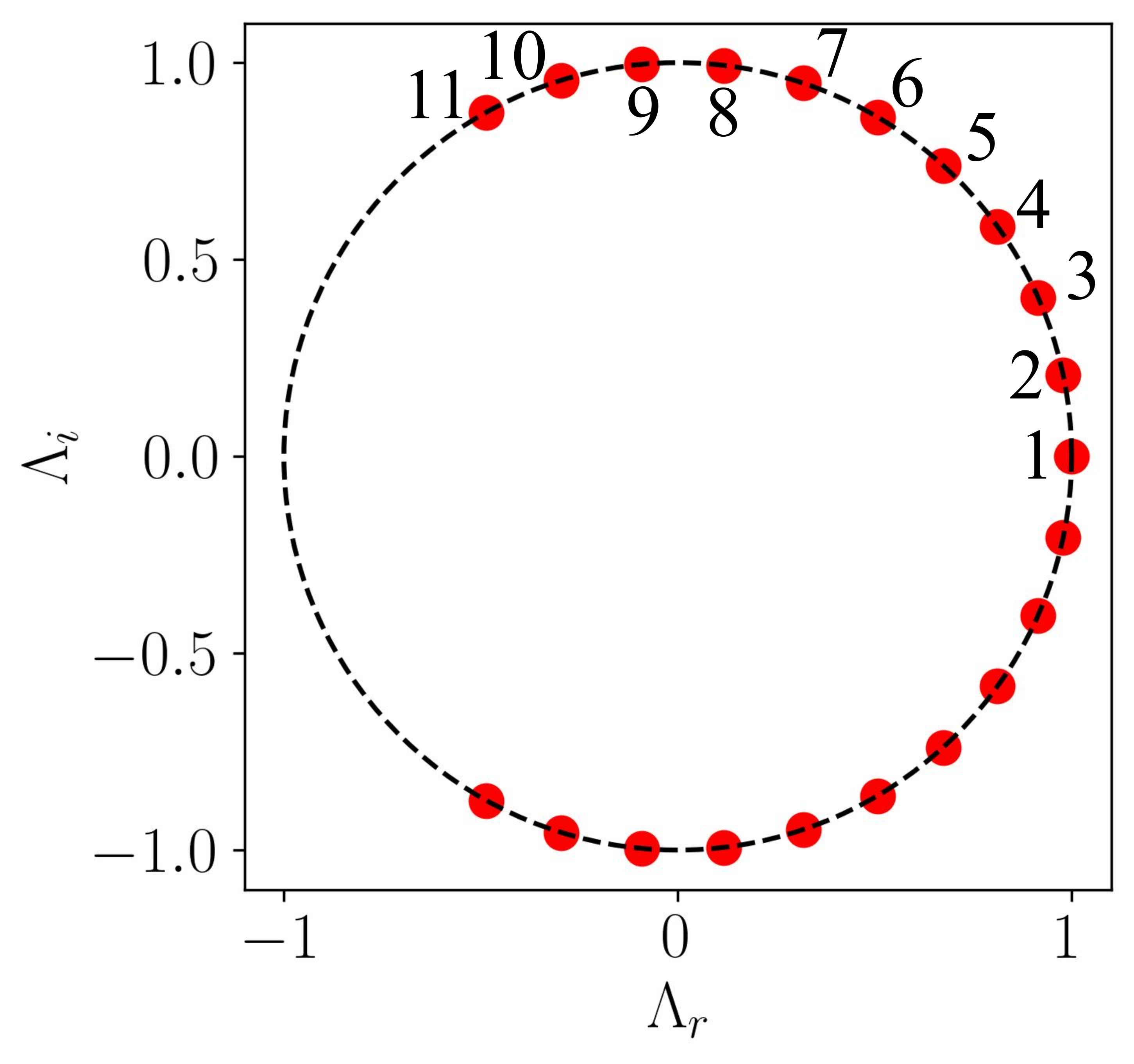
In this plot, all points lie on the unit circle, indicating that the modes neither grow nor decay, signifying stable DMD modes. This aligns with our chosen scenario, where the flow around a circular cylinder at Re = 100 exhibits stable periodic vortex shedding.
Now, utilizing simple plotting routines, we can visualize the DMD modes:
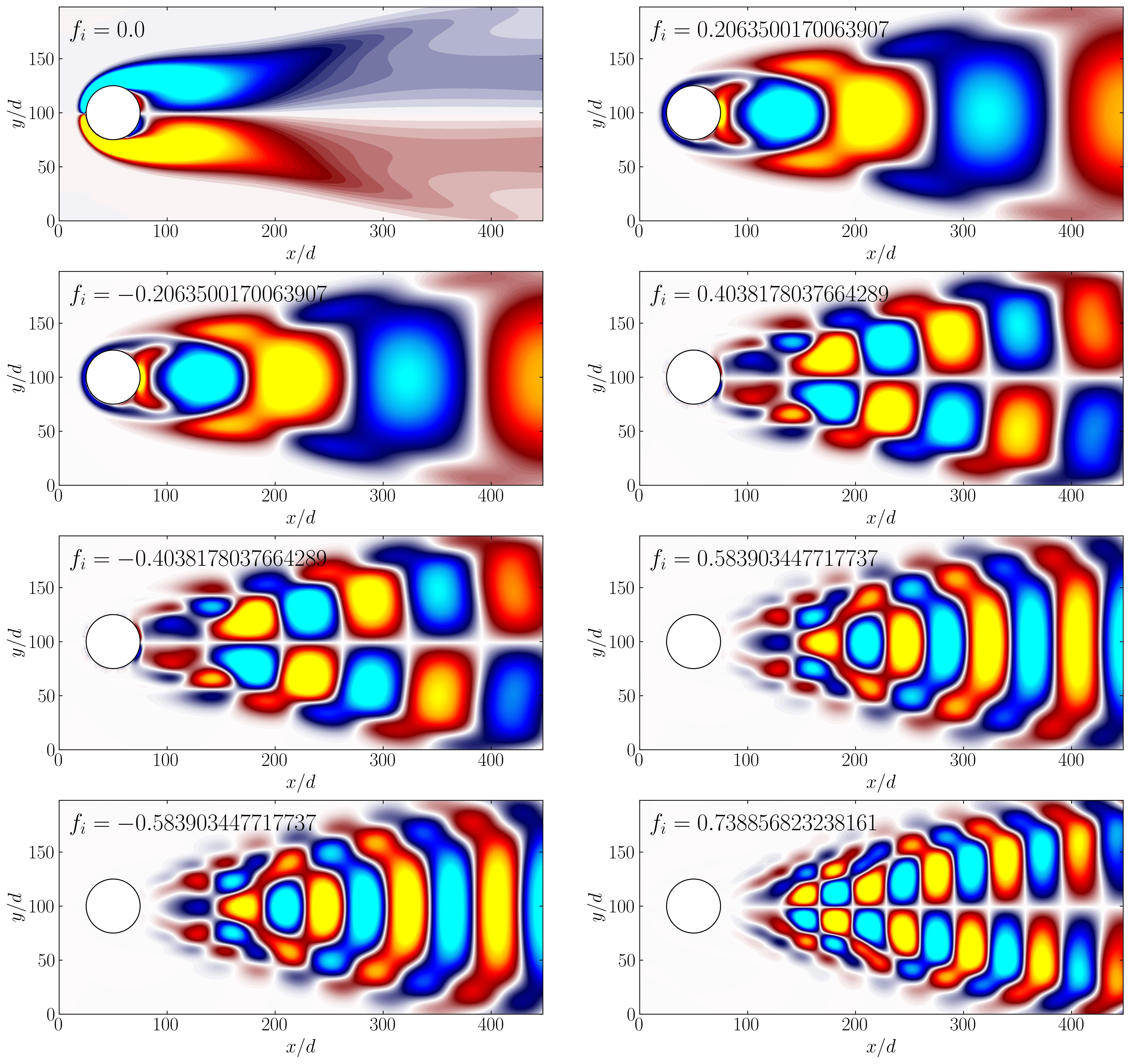
Unlike POD, DMD not only provides modes but also a set of associated eigenvalues, establishing a low-dimensional dynamical system governing the evolution of mode amplitudes over time. Furthermore, unlike POD, the mean is not subtracted in the DMD calculation, and the first mode (f = 0) corresponds to a background mode that remains unchanged (i.e., it possesses a zero eigenvalue). The DMD modes resemble the POD modes in this example because POD furnishes a harmonic decomposition, resulting in modal amplitudes that are roughly sinusoidal over time at harmonic frequencies of the dominant vortex shedding.
Lastly, the rank-21 reconstruction of the flow field bears resemblance to the original flow field, as depicted below:
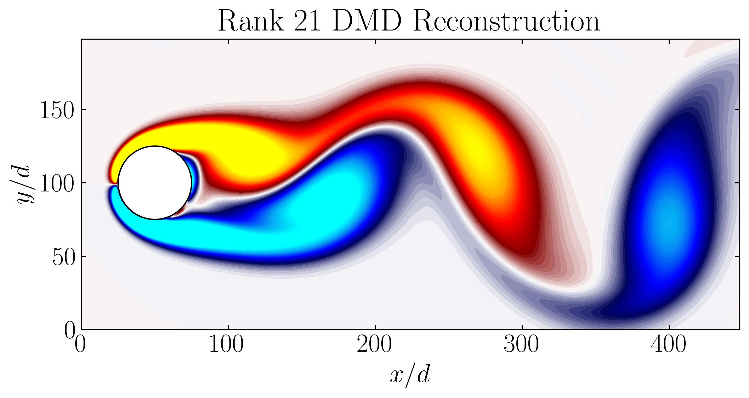
In conclusion, Dynamic Mode Decomposition emerges as a powerful tool for uncovering dominant dynamics within fluid systems, offering insights into both mode structures and their temporal evolution. In our exploration, we’ve witnessed its efficacy in capturing stable modes within the wake behind a circular cylinder. In the next article, we’ll focus on the application of DMD using OpenFOAM simulation data, extending our understanding of its capabilities in real-world fluid dynamics scenarios.
Enjoy Reading This Article?
Here are some more articles you might like to read next: