Unlocking the secrets within your OpenFOAM data goes beyond just post-processing numbers. Modal decomposition methods offer a powerful lens to analyze your simulations, revealing hidden patterns and dominant flow features. This guide will equip you with the knowledge to set up an OpenFOAM case specifically designed for modal decomposition analysis, empowering you to extract deeper insights from your CFD simulations.

Have you ever felt limited by the sheer volume of data generated by your OpenFOAM simulations? While the data holds valuable insights, extracting meaningful information can feel overwhelming. Here’s where modal decomposition methods step in! These powerful techniques offer a way to analyze your data through the lens of its dominant modes, revealing hidden patterns and providing a deeper understanding of the underlying flow phenomena. Proper Orthogonal Decomposition (POD), Dynamic Mode Decomposition (DMD), Spectral Proper Orthogonal Decomposition (SPOD), and Bi-spectral Mode Decomposition (BMD) are the main modal decomposition methods that we aim to test.

This blog post will guide you through setting up an OpenFOAM case specifically tailored for modal decomposition analysis. We’ll delve into the key considerations for data extraction and preparation, ensuring your data is optimized for unlocking the power of these methods. By the end, you’ll be equipped to bridge the gap between raw simulation data and insightful interpretations, allowing you to gain a richer understanding of your fluid dynamics simulations.

Lets begin!!!

Problem Description

To facilitate the exploration of various modal decomposition techniques, we will focus on the dynamics of a two-dimensional flow around a square cylinder at a Reynolds number of 100. The flow will be simulated using Direct Numerical Simulations (DNS) implemented in OpenFOAM. The setup of this case will closely adhere to the configuration outlined by Bai and Alam (2018) for reference. A visual representation of the domain is provided below:

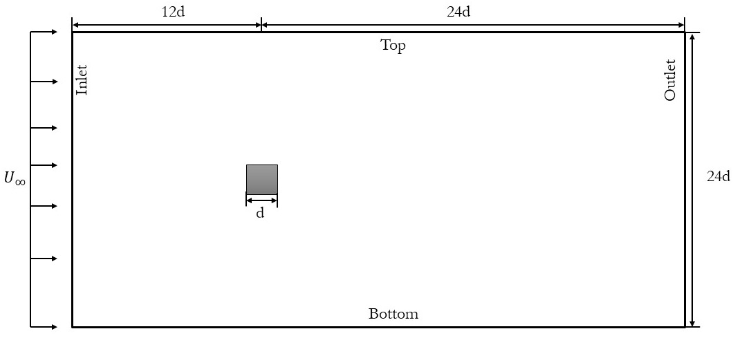
The choice of this specific case is deliberate. The wake generated behind the cylinder is a classic example of periodic (Kármán) vortex shedding. This phenomenon manifests as a repetitive shedding of vortices, resulting in a periodic flow regime characterized by a dominant frequency and its harmonics. These inherent characteristics render it an ideal candidate for modal decomposition investigations. Moreover, by replicating a published case, we can effectively scrutinize and validate the underlying flow physics within our simulations.

Numerical setup : 0

Once the domain is established, proceed to generate a mesh using your preferred mesher. Since this is a 2D scenario, the mesh should be feasible for computation on a standard PC with 8-12 threads. Moving forward, let’s configure the boundary conditions.

At the inlet boundary, enforce a uniform streamwise velocity (designated as $U_\infty$), while employing a pressure-outlet boundary condition at the outlet. The no-slip condition must be imposed on the surface of the cylinder. The top and bottom boundaries will be treated as slip sides, utilizing symmetric conditions. In OpenFOAM, for the 2D case, it’s necessary to specify the front and back boundaries as either empty or as slip sides with symmetric conditions. Given that this is a laminar (DNS) case, our focus will be solely on setting up boundary conditions for velocity and pressure.

For those seeking guidance on configuring an unsteady case in OpenFOAM, refer to the link provided here.

Tip: Start with a basic pitzDaily case in OpenFOAM and adapt the necessary files to suit your specific case.

The boundary conditions for velocity in the Case/0/U file will be as follows:

internalField   uniform (0.015 0 0);
boundaryField
{
    TOP
    {
        type                      slip;
    }
    BOTTOM
    {
        type                      slip;
    }
    SIDE1
    {
        type                      slip;
    }
    SIDE2
    {
        type                      slip;
    }
    INLET
    {
        type                      fixedValue;
        value                     uniform (0.015 0 0);
    }
    OUTLET
    {
        type                      zeroGradient;
    }
    PRISM
    {
        type                      noSlip ;
    }
}

The boundary conditions for pressure in Case/0/p file will be as follows:

internalField   uniform 0;
boundaryField
{
    TOP
    {
        type                      zeroGradient;
    }
    BOTTOM
    {
        type                      zeroGradient;
    }
    SIDE1
    {
        type                      zeroGradient;
    }
    SIDE2
    {
        type                      zeroGradient;
    }
    INLET
    {
        type                      zeroGradient;
    }
    OUTLET
    {      
        type                       fixedValue;
        value                      uniform 0;
    }
    PRISM
    {
        type                      zeroGradient ;
    }
}

Numerical setup : constant

Next, we’ll configure the constant folder within your case. There are two key aspects to consider: the flow will be Newtonian, and we’ll be employing Direct Numerical Simulations (DNS), indicating a laminar case.

Modify the constant/turbulenceProperties file as follows:

simulationType  laminar;

And update the constant/transportProperties file to reflect the Newtonian fluid model:

transportModel  Newtonian;

nu              [0 2 -1 0 0 0 0] 0.000015;

Numerical setup : system

The system folder serves as the locus for configuring the numerical setup of your case. As we embark on the exploration of modal decomposition techniques such as Proper Orthogonal Decomposition (POD), Dynamic Mode Decomposition (DMD), Spectral Proper Orthogonal Decomposition (SPOD), and Bi-spectral Mode Decomposition (BMD), several considerations warrant attention:

• Achieving Fully Developed Flow: Before commencing data collection, it’s imperative to ensure that the flow within the domain reaches a fully developed state. This entails allowing sufficient time for transient effects to dissipate, ensuring that the flow attains a stable and representative behavior.
• Snapshot Data Collection: Data collection should be structured around capturing snapshots or time instances of the flow field. These snapshots serve as the foundation for subsequent analysis and decomposition techniques, facilitating a comprehensive understanding of the flow dynamics.
• Verification and Validation Probes: Incorporating probes within the domain enables the verification and validation of the simulated results against established literature or experimental data. These probes serve as reference points, aiding in assessing the accuracy and fidelity of the computational model.

Let’s delve deeper into each of these aspects to elucidate their significance in the context of modal decomposition investigations.

Fully developed flow

Achieving a fully developed flow entails reaching a state where the flow characteristics stabilize and no longer vary with increased distance. In our case, where we anticipate a periodic vortex shedding phenomenon, our objective is to attain a fully developed periodic flow field. This implies running the simulation until the flow becomes statistically stationary or stable, devoid of random fluctuations or variations. A visual representation of this phenomenon might resemble the following:

To accomplish this, we’ll initially run the simulation for a duration equivalent to 20 Through Times. Through Time represents the duration a fluid particle requires to traverse the domain length undisturbed, calculated as:

This ensures that we accumulate sufficient data to capture a converged transient solution, thereby setting the system/constant/endTime parameter appropriately.

libs (petscFoam);

application     pimpleFoam;

startFrom       latestTime;//startTime;

startTime       0;

stopAt          endTime;

endTime         4800; // 20 Through times

deltaT          0.01;

writeControl    timeStep;

writeInterval   4600;

purgeWrite      0;

writeFormat     ascii;

writePrecision  8;

writeCompression on;

timeFormat      general;

timePrecision   8;

runTimeModifiable true;

To calculate the time step, denoted as $\Delta t$, we aim for a Courant-Friedrichs-Lewy (CFL) number of $\leq 0.8$ to ensure stability in our simulations. With knowledge of the minimum element size ($\Delta x$) and the free-stream velocity ($U_{ref}$), the time step can be estimated as follows:

This value is then assigned to deltaT in the controlDict file. By adhering to this criterion, we ensure that our time discretization is sufficiently fine to capture the dynamics of the flow accurately while maintaining numerical stability.

Snapshot data collection

Now, let’s delve into the data collection process crucial for modal decomposition analysis. We aim to capture multiple snapshots of the flow field, each representing a distinct time instance. Following established standards in the literature, we’ll need $2^n$ snapshots, where 𝑛 can be user-specific and case-specific. For this particular case, we’ll extract between 256 to 1024 snapshots.

However, this data collection can only commence after reaching a fully developed, statistically stable flow. Hence, any data collection occurs after the endTime specified in the setup earlier.

There are two approaches to collect snapshot data:

1. Utilizing writeControl to save multiple time directories.
2. Extracting required slices or surfaces using the surfaces function object.

For the first method, after running the simulation for 20 Through Times, rerun the simulation with writeControl set to timeStep in the controlDict file. Regarding the writeInterval, let’s refer back to the flow physics as documented in Bai and Alam (2018). They report a dominant Strouhal number of 0.146 for the case of flow around a square cylinder at Reynolds number 100. This implies a shedding cycle time of approximately 46 seconds or 4600 time steps. Since we aim to extract data spanning at least 10 shedding cycles (46000 time steps) with 16-32 data points in each cycle, the writeInterval should be set to 287. Ensure purgeWrite is disabled (set to 0) and adjust the endTime accordingly to encompass 10 vortex shedding cycles. Then, execute the simulation to obtain the requisite data.

For the second method, we’ll leverage functionObjects within OpenFOAM to extract 2D slices positioned at the symmetric mid-point of our domain. This can be achieved using the surfaces function object as demonstrated below:

surfaces
{
    type            surfaces;
    libs            ("libsampling.so");
    writeControl   	timeStep;
    writeInterval   285;

    surfaceFormat   vtk;
	
	formatOptions
	{
		vtk
		{
			legacy true;
			format ascii;
		} 
	}
	
    fields          (p U);

    interpolationScheme cellPoint;

    surfaces
    {
        zNormal
        {
            type        cuttingPlane;
            point       (0 0 0);
            normal      (0 0 1);
            interpolate true;
        }
    };
};

Validation

To validate our setup against the case of Bai and Alam (2018), we’ll compare the Strouhal number and mean drag and lift coefficients obtained from our numerical simulation with their study. To begin, we’ll position multiple probes within our domain to extract velocity and pressure downstream of the cylinder, where vortex shedding is prominent. We’ll employ the probes function object for this purpose, as illustrated below:

probes
{
    type            probes;
    libs            ("libsampling.so");

    // Name of the directory for probe data
    name            probes;

    // Write at same frequency as fields
    writeControl    timeStep;
    writeInterval   1;

fields (
        p 
        U 
       );

probeLocations
(

	(0.15 0.05 0)
	(0.15 0 0)
	(0.15 -0.05 0)
	
	(0.35 0.1 0)
	(0.35 0.05 0)
	(0.35 0 0)
	(0.35 -0.05 0)
	(0.35 -0.1 0)
	
	(0.55 0.1 0)
	(0.55 -0.05 0)
	(0.55 0 0)
	(0.55 -0.05 0)
	(0.55 -0.1 0)
	
);
    // Optional: filter out points that haven't been found. Default
    //           is to include them (with value -VGREAT)
    includeOutOfBounds  true;
}

To extract the drag and lift coefficients, utilize the forceCoeffs function object as depicted below:

forces
    {
        type            forceCoeffs;
        libs ( "libforces.so" );
    
        writeControl   timeStep;
        writeInterval  1;
        
        patches         ( "PRISM" );
        
        rho             rhoInf;
        log             true;
        rhoInf          1.225;
        liftDir         (0 1 0);
        dragDir         (1 0 0);
        //sideDir         (0 0 1);
        CofR            (0 0 0);
        pitchAxis       (0 0 1);
        magUInf         0.015;
        lRef            0.1;
        Aref            0.01;
    }

Next, we’ll extract velocity and pressure signals from the probes and compute the fast Fourier transform to determine the dominant Strouhal number of the vortex shedding process, comparing it with published data. Subsequently, we’ll compute the time-average of the drag and lift coefficient data and perform a similar comparison. For guidance on post-processing using Python, refer to my previous article.

Following these instructions, your case will be primed for investigation using any modal decomposition methods. You can find a reference case setup for the flow around a square cylinder at Reynolds number 100 here.