Fluid flow can be a swirling mystery, but fear not! Proper Orthogonal Decomposition (POD) can help us see through the chaos. POD acts like a magnifying glass for fluid dynamics, allowing us to extract the key, recurring patterns, or “coherent modes,” hidden within complex data. This post will explain how POD works and how it empowers us to understand and predict complex flow behavior.

In the vast seas of fluid dynamics, where currents swirl, eddies dance, and turbulence reigns supreme, lies a powerful tool capable of unraveling the intricate mysteries of flow behavior. Welcome to the realm of Proper Orthogonal Decomposition (POD), a methodological masterpiece revered by scientists and engineers alike for its ability to distill complex fluid phenomena into manageable insights.

Picture this: a turbulent river, its surface rippling with chaotic motion, seemingly unpredictable to the untrained eye. Understanding and predicting such flows is akin to deciphering a cryptic language, where every swirl, every eddy, holds a story of its own. Here steps in POD, a beacon of clarity amidst the turbulence, offering a structured approach to unraveling the hidden patterns within.

In this blog post, we embark on a journey through the depths of fluid dynamics, guided by the principles and applications of Proper Orthogonal Decomposition. We’ll delve into its origins, unravel its mathematical underpinnings, and explore its diverse array of applications across various fields—from aerospace engineering to environmental science.

But before we plunge into the intricacies of POD, let’s pause for a moment to reflect on the fundamental question: What exactly is proper orthogonal decomposition, and why does it hold such sway over the realm of fluid dynamics? At its core, POD is not merely a technique; it’s a philosophy—a way of thinking that seeks order amidst chaos, seeking simplicity in complexity. By decomposing complex flow fields into a set of orthogonal modes ordered by their energy content, POD unveils the underlying structures governing fluid motion, shedding light on coherent structures, dominant patterns, and hidden dynamics that elude the naked eye.

Join me as I embark on this odyssey, where mathematical elegance meets the turbulent beauty of fluid flows. Lets begin!!

History

The Proper Orthogonal Decomposition (POD) stands as one of the most widely used data analysis and modeling techniques in fluid mechanics. Its prevalence over the last half-century has paralleled advancements in experimental measurement methods, the rapid evolution of computational fluid dynamics, theoretical progress in dynamical systems, and the increasing capacity to handle and process vast amounts of data. At its essence, POD involves applying Singular Value Decomposition (SVD) to a dataset with its mean subtracted (PCA), making it a cornerstone dimensionality reduction method for investigating intricate, spatio-temporal systems.

These systems typically manifest through nonlinear dynamical equations governing the evolution of quantities of interest across time and space within physical, engineering, or biological domains. The efficacy of POD stems from the recurring observation that meaningful behaviors in most complex systems are encoded within low-dimensional patterns of dynamic activity. Leveraging this insight, the POD technique aims to construct reduced-order models (ROMs) that capture the essential dynamics of the underlying complex system.

In particular, Reduced Order Models (ROMs) utilize POD modes to map complex systems, such as turbulent flows, onto lower-dimensional subspaces. Within these subspaces, simulations of the governing model become more tractable and computationally efficient, enabling more accurate evaluations of the system’s spatiotemporal evolution.

Origins

Suppose we have a dataset, denoted as $y(x,t)$, which is a function of both space and time. Let’s consider that this dataset depicts the phenomenon of vortex shedding behind a cylinder or the flow around a car. When analyzing such a dataset, the initial imperative is to grasp its key characteristics, including the fundamental dynamics governing its formation. To achieve this, one can begin by decomposing the data into two distinct variables, as follows:

Here, we’ve decomposed the data into a sum of spatial modes, denoted as φ(x), and their time-varying coefficients or temporal modes, represented by a(t). While there are several methods available for such decomposition, such as performing Fourier transforms in both space and time to obtain a Fourier basis for the system, POD distinguishes itself by opting for a data-driven decomposition.

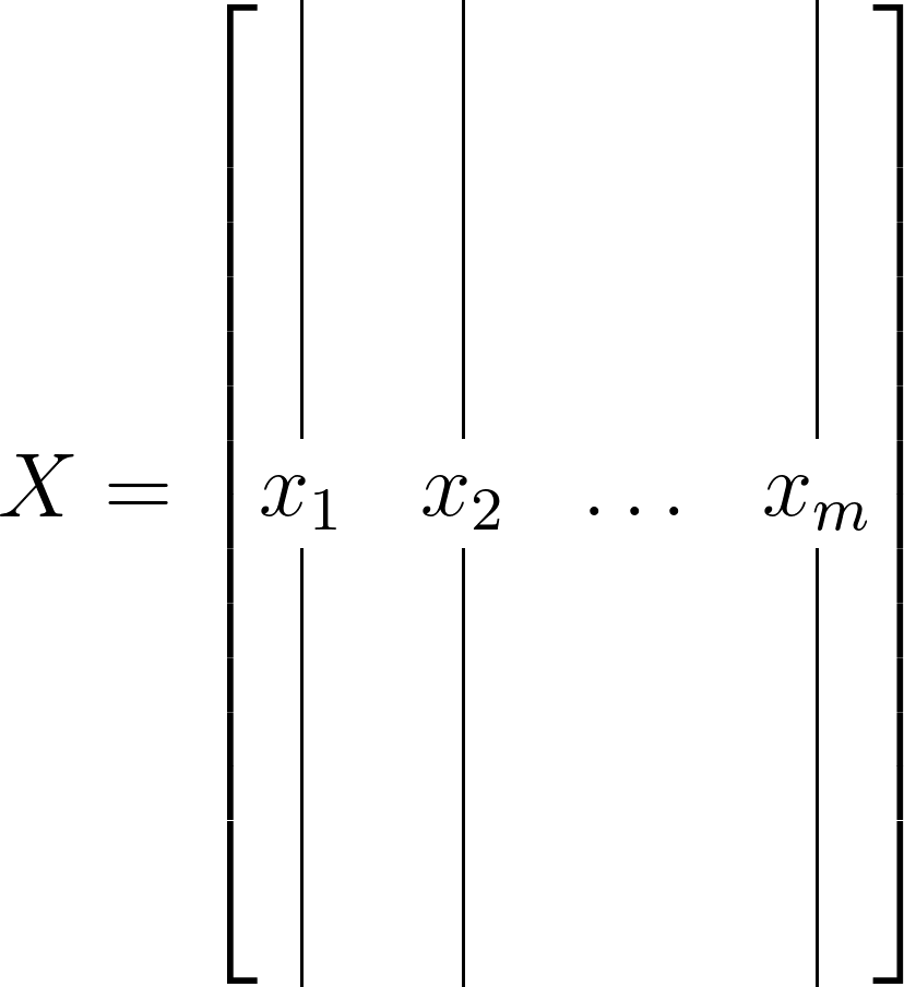
In essence, POD can be conceptualized as the outcome of applying SVD to a suitably arranged data matrix. Consequently, many properties of POD directly stem from those of SVD. Consider a matrix X with n rows and m columns. In most instances, X will be a tall and slender data matrix, like so:

Now, let’s assume that the matrix X is an r-rank matrix, where r ≤ min(m,n). In this scenario, the reduced singular value decomposition of X can be defined as follows:

where, Φ is of size n×r, Ψ is of size m×r, and Σ of r×r. Here, Σ is a diagonal matrix comprising the singular values, while Φ consists of the singular vectors. One can perceive the singular values akin to eigenvalues (Σ) and the singular vectors akin to eigenvectors (Φ). Moreover, Φ and Ψ are orthonormal matrices, ensuring the following orthogonality property:

Here, I represents an identity matrix, and the * symbol denotes the adjoint or conjugate transpose of a matrix. This process illustrates the method of obtaining a reduced or truncated SVD of X. It’s important to note that SVD exists for any and all matrices, whereas eigenvalue decomposition is only possible for square matrices.

Proper Orthogonal Decomposition

Proper Orthogonal Decomposition (POD) finds its roots intertwined with two fundamental concepts in mathematics and statistics: Singular Value Decomposition (SVD) and the covariance matrix. SVD, a cornerstone of linear algebra, provides the theoretical backbone upon which POD stands, enabling the decomposition of complex data into its essential components. Meanwhile, the covariance matrix serves as a bridge between the raw data and the orthogonal modes unearthed by POD, encapsulating the statistical relationships and variability within the dataset. Together, these concepts form the bedrock upon which POD flourishes, offering a systematic framework for unraveling the rich tapestry of fluid dynamics.

Suppose we are gathering data that varies with both space and time, and we assemble it into a matrix where the columns represent time (referred to as snapshots) and the rows represent spatial locations at individual time instances. Let’s revisit the example of flow around a cylinder and presume we’re measuring the fluid velocity (u and v) at various spatial points (x1, x2, …, xn) and time intervals (t1, t2, …, tm). In this scenario, the matrix takes the form of an n×m matrix:

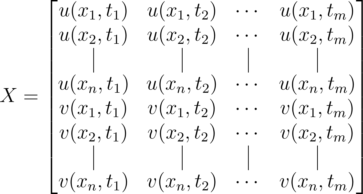
Here, the dimensionality of the matrix is doubled to 2n since we have two velocity measurements at each spatial location. It’s important to note that we’re not making any assumptions about the spatial or temporal resolution of our data, nor about the specific quantity or quantities being measured. The only implicit assumption we’re making in constructing X is that we measure the same quantities for each snapshot.

Given that X captures the transient behavior of a system, such as fluid flow in this case, we can subtract the time-averaged dataset from each column of X to derive a mean-removed matrix, denoted as Y:

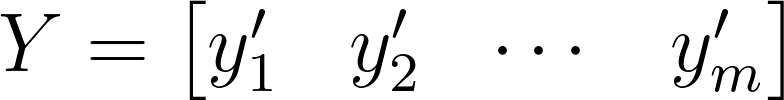
In this case, the jth mean-removed snapshot would be expressed as:

Lastly, the Proper Orthogonal Decomposition (POD) can be obtained by simply performing the Singular Value Decomposition (SVD) on the mean-removed matrix Y, as shown below:

In this instance, the POD modes are represented by the columns of $\phi(x)$ within the matrix $\Phi$, which evolve over time through the associated time-coefficients $a(t)$, as depicted by:

The POD expansion of the data is expressed through the dyadic expansion of the SVD, illustrated by:

Properties

• Data arrangement: Spatial location depends only on row number, while temporal location depends only on the column.
• Separation of variables: Left and right singular vectors correspond to space and time, respectively, facilitating the direct use of Singular Value Decomposition (SVD) for data analysis.
• Optimality property of SVD: Truncating the SVD sum to r terms provides the closest rank-r approximation to the full dataset.
• Flexibility in data arrangement: Changing the order of measurements, such as placing velocity components u and v in alternating rows, does not affect the SVD decomposition. Rearranging columns also has no impact on the Proper Orthogonal Decomposition (POD) modes.
• Permutation properties: Rearranging data does not alter the POD modes except for permuting entries to appropriate locations.
• Time-resolved data: Shuffling the order of time-resolved snapshots does not affect the POD modes, demonstrating that POD does not necessarily require time-resolved data and can handle non-time-resolved sequences effectively.

Importance of correlation matrix

Utilizing the mean-removed matrix Y, we can establish two significant correlations. The first correlation is derived by computing the spatial inner product (column-wise correlation), denoted as $Y^Y$, while the second correlation is obtained by calculating the inner product along the time dimension (row-wise correlation), denoted as $YY^$. Both of these correlations are demonstrated below:

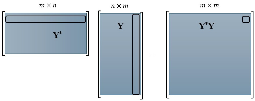
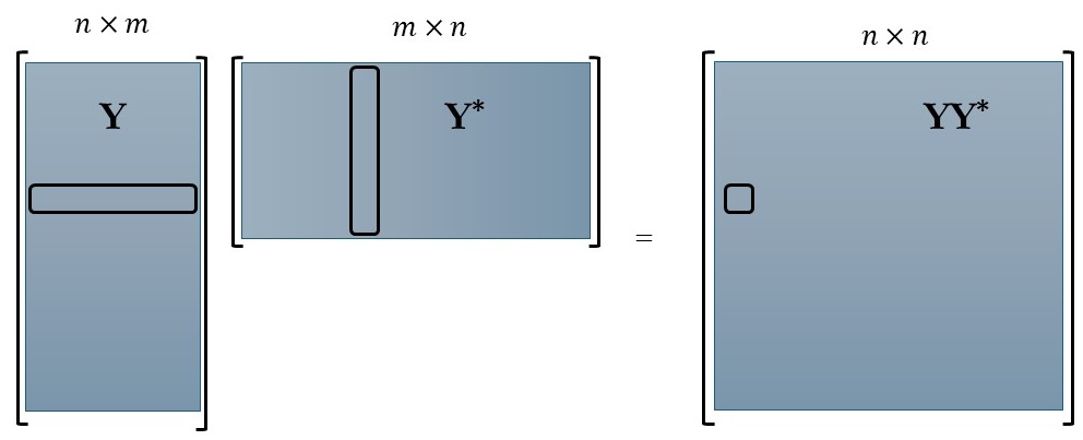
In accordance with the POD equation, the right-singular vectors (Ψ) correspond to the eigenvectors of the matrix $Y^Y$, while the left-singular vectors (Φ) correspond to the eigenvectors of $YY^$. For reference, here is the mathematical representation:

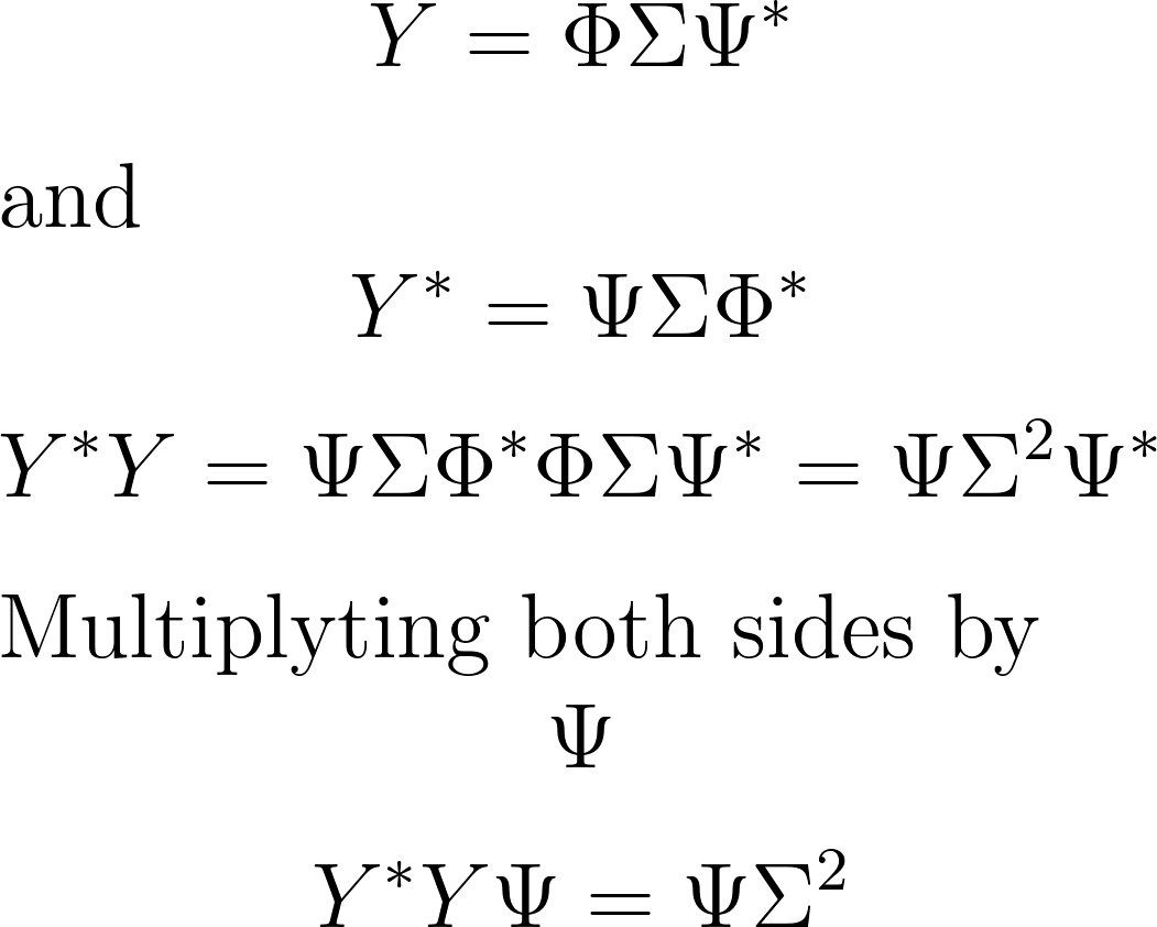
The final equation essentially transforms into the eigenvalue decomposition of $Y^*Y$, where $\Psi$ serves as the eigenvectors and $\Sigma$ represents the square root of the eigenvalues. A similar interpretation applies to the row-wise correlation matrix.

It’s worth noting that the two matrices $YY^\ast$ and $Y^\ast Y$ typically have different dimensions, with $YY^\ast$ being $n\times n$ and $Y^\ast Y$ being $m\times m$. Given that the SVD of Y is linked to the eigendecompositions of these square matrices, it’s often more convenient to compute and manipulate the smaller of the two matrices. For instance, if the spatial dimensions in each snapshot are extensive while the number of snapshots is relatively small ($m\ll n$), it may be more manageable to compute the (full or partial) eigendecomposition of $Y^\ast Y$ to obtain the POD coefficients $a(t)$. Conversely, if $n\ll m$, one could instead initiate the process by computing an eigendecomposition of $YY^\ast$.

In summary, we delved into the mathematical underpinnings of Proper Orthogonal Decomposition (POD), unraveling its intricacies from interpreting correlation matrices to leveraging eigenvalue decompositions. Our exploration sheds light on the mechanics of POD. In the upcoming article, we shift our focus to the practical application of POD. By utilizing the flow around a cylinder dataset from Data-Driven Modeling of Complex Systems, we aim to elucidate how POD operates in real-world scenarios. This examination will underscore its versatility in capturing fundamental dynamics and streamlining computational complexity.

Until next time!