Continuing our exploration of POD, we delve into the Method of Snapshots. This powerful technique analyzes fluid behavior, like flow around a cylinder, by capturing “snapshots” of the flow field at different times. With these snapshots, POD can identify key flow features and unlock hidden patterns, providing deeper insights into seemingly chaotic fluid dynamics.

In the vast and ever-evolving landscape of fluid dynamics, understanding the complex interplay of flows is paramount. Imagine a turbulent river, its currents twisting and turning with seemingly chaotic abandon, or a supersonic aircraft slicing through the atmosphere, leaving a trail of intricate vortices in its wake. Deciphering such intricate phenomena requires more than mere observation; it demands a systematic approach that can distill the essence of motion from the chaos.

Enter Proper Orthogonal Decomposition (POD)—a beacon of clarity amidst the turbulence—a methodological masterpiece that has revolutionized the study of fluid dynamics. In our previous exploration, we delved into the mathematical foundations of POD, unraveling its elegant principles and uncovering the mathematical machinery that powers this transformative tool. Now, armed with this mathematical arsenal, we embark on a new expedition, diving deeper into the practical applications of POD, with a particular focus on the Method of Snapshots.

Check out my previous article on the basics of POD here.

The Method of Snapshots stands as one of the most potent techniques in the POD toolkit, offering a pragmatic approach to capturing the dynamic behavior of fluid flows. Unlike traditional analytical methods, which often struggle to cope with the complexity of real-world phenomena, the Method of Snapshots embraces the richness of empirical data, harnessing the power of observation to uncover hidden patterns and structures within. In this blog post, we navigate the intricate waters of fluid dynamics, guided by the Method of Snapshots as our compass. We’ll explore how this approach leverages a collection of discrete snapshots—time-resolved observations of flow fields—to construct a comprehensive representation of fluid behavior. We will utilize the flow around a cylinder dataset from Data-Driven Modeling of Complex Systems. From turbulent eddies to coherent structures, each snapshot serves as a glimpse into the intricate dance of fluid motion, capturing moments frozen in time that collectively unveil the underlying dynamics at play.

But before we plunge into the depths of the Method of Snapshots, let’s take a moment to reflect on its significance within the broader framework of POD. At its core, POD seeks to decompose complex flow fields into a set of orthogonal modes, ordered by their energy content—a task made possible by the Method of Snapshots’ ability to extract meaningful information from observational data. By leveraging this empirical approach, we can bypass the limitations of traditional modeling techniques, embracing the inherent complexity of fluid flows with unparalleled fidelity.

Lets begin!

Method of Snapshots

When the data matrix, X, exceeds the capacity of system memory, employing the method of snapshots becomes preferable for POD analysis. The method of snapshots discretizes the POD procedure within the temporal domain. Let’s envision the data matrix X, comprising velocity field (u and v) measurements gathered across different spatial points ($x_1, x_2, …, x_n$) and time intervals ($t_1, t_2, …, t_m$):

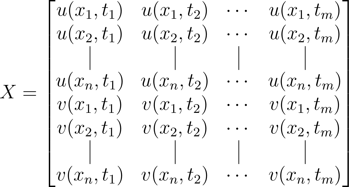
When the matrix becomes too large for system memory due to the extensive spatial degrees of freedom (n) compared to the number of snapshots (m), a practical solution is to create the column-wise covariance matrix ($Y^\ast Y$). This correlation matrix, sized m×m, proves highly memory-efficient compared to the original matrix. Subsequently, applying SVD to this covariance matrix enables the extraction of eigenvectors and eigenvalues.

Here’s a systematic approach for the method of snapshots:

1. Form the data Matrix X:

Start by assembling your dataset into a matrix X. This matrix represents your data, where each column corresponds to a snapshot in time and each row represents a different spatial location or measurement.

2. Obtain the mean-removed matrix Y:

Subtract the time-averaged data from each column of X to obtain the mean-removed matrix Y. This process helps to remove the average behavior or trends from the data, focusing instead on the deviations or fluctuations around the mean.

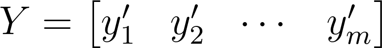
The jth term of the mean-removed matrix Y represents the deviation of the jth snapshot from the time-averaged data.

3. Form the covariance matrix using Y:

Calculate the covariance matrix using the mean-removed matrix Y. The covariance matrix provides a measure of how two variables change together. Each element of the covariance matrix represents the covariance between two different snapshots, capturing the relationships between different time instances in the data.

4. Apply SVD to the covariance matrix:

Utilize Singular Value Decomposition (SVD) on the covariance matrix obtained in the previous step. SVD decomposes the covariance matrix into three matrices: U, Σ, and $V^\ast$, where U contains the left singular vectors, Σ is a diagonal matrix containing the singular values, and V* contains the right singular vectors.

5. Obtain the POD modes:

The POD modes are extracted from the SVD of the covariance matrix. These modes are obtained from the columns of the left singular vectors matrix U, corresponding to the dominant modes of variation in the dataset.

POD on flow around cylinder

As promised in the previous article, we will now apply the method of snapshots to perform Proper Orthogonal Decomposition (POD) on the flow field around a circular cylinder. To do this, we’ll utilize the flow around a cylinder dataset available from Data-Driven Modeling of Complex Systems. Begin by downloading the dataset from here.

Next, fire up a Jupyter notebook and follow along. Let’s start by importing some essential modules:

import matplotlib.colors
import matplotlib.pyplot as plt
import numpy as np
import pandas as pd
import scipy as sp
import os
import imageio
import io

%matplotlib inline

plt.rcParams.update({'font.size' : 18, 'font.family' : 'Times New Roman', "text.usetex": True})

Next, proceed to set the paths for your data files (the one you downloaded) and the save locations. This ensures that your code can access the dataset and saves any outputs to the desired locations.

Path = 'E:/Blog_Posts/BruntonCylinder/'
save_path = 'E:/Blog_Posts/OpenFOAM/ROM_Series/Post22/'
Files = os.listdir(Path)
print(Files)

### OUTPUT
### ['CYLINDER_ALL.mat']

Load the CYLINDER_ALL.mat:

Contents = sp.io.loadmat(Path + Files[0])

Given that this file essentially acts as a dictionary, you can list out its keys using the keys() method:

Contents.keys()

### Output:
### dict_keys(['__header__', '__version__', '__globals__', 'UALL', 'UEXTRA', 'VALL', 'VEXTRA', 'VORTALL', 'VORTEXTRA', 'm', 'n', 'nx', 'ny'])

Let’s begin by extracting the necessary data from this dictionary. This step involves identifying and retrieving the specific information or variables needed for our analysis.

m = Contents['m'][0][0]
n = Contents['n'][0][0]
Vort = Contents['VORTALL']
print(m, n)
print(Vort.shape)

### Output:
### 199 449
### (89351, 151)

Based on this information, we understand that the data comprises 199 x 499 (= 89,351) spatial degrees of freedom and includes 151 available snapshots. Let’s proceed by visualizing one snapshot to gain a clearer understanding of the dataset we’re working with.

Circle = plt.Circle((50, 100), 25, ec='k', color='white', zorder=2)

fig, ax = plt.subplots(figsize=(11, 4))

p = ax.contourf(np.reshape(Vort[:,0],(n,m)).T, levels = 1001, vmin=-2, vmax=2, cmap = cmap.reversed())
q = ax.contour(np.reshape(Vort[:,0],(n,m)).T, 
               levels = [-2.4, -2, -1.6, -1.2, -0.8, -0.4, -0.2, 0.2, 0.4, 0.8, 1.2, 1.6, 2, 2.4], 
               colors='k', linewidths=1)
ax.add_patch(Circle)
ax.xaxis.set_tick_params(direction='in', which='both')
ax.yaxis.set_tick_params(direction='in', which='both')
ax.xaxis.set_ticks_position('both')
ax.yaxis.set_ticks_position('both')
ax.set_aspect('equal')

ax.set_xlabel(r'$\bf x/d$')
ax.set_ylabel(r'$\bf y/d$')

plt.show()

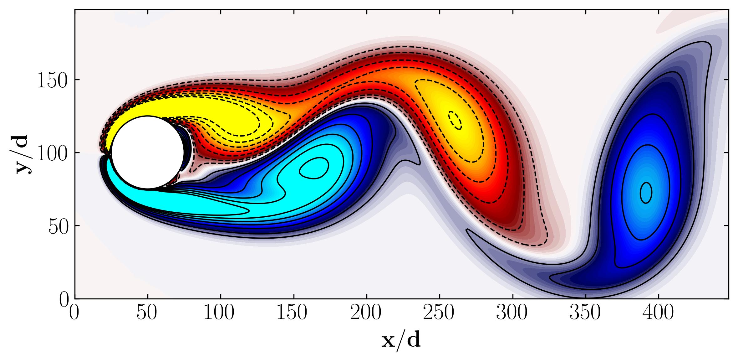
Here, we’re examining a vorticity field dataset, as depicted above. Vorticity represents the curl of velocity and essentially illustrates any twisting or swirling motion within the flow. Given that we’ve encompassed all velocity-related aspects through the vorticity field, we’re now equipped to carry out Proper Orthogonal Decomposition (POD) on this dataset.

### Data Matrix
X = Vort

### Mean-removed Matrix
X_mean = np.mean(X, axis = 1)
Y = X - X_mean[:,np.newaxis]

### Covariance Matrix
C = np.dot(Y.T, Y)/(Y.shape[1]-1)

### SVD of Covariance Matrix
U, S, V = np.linalg.svd(C)

### POD modes
Phi = np.dot(Y, U)

### Temporal coefficients
a = np.dot(Phi.T, Y)

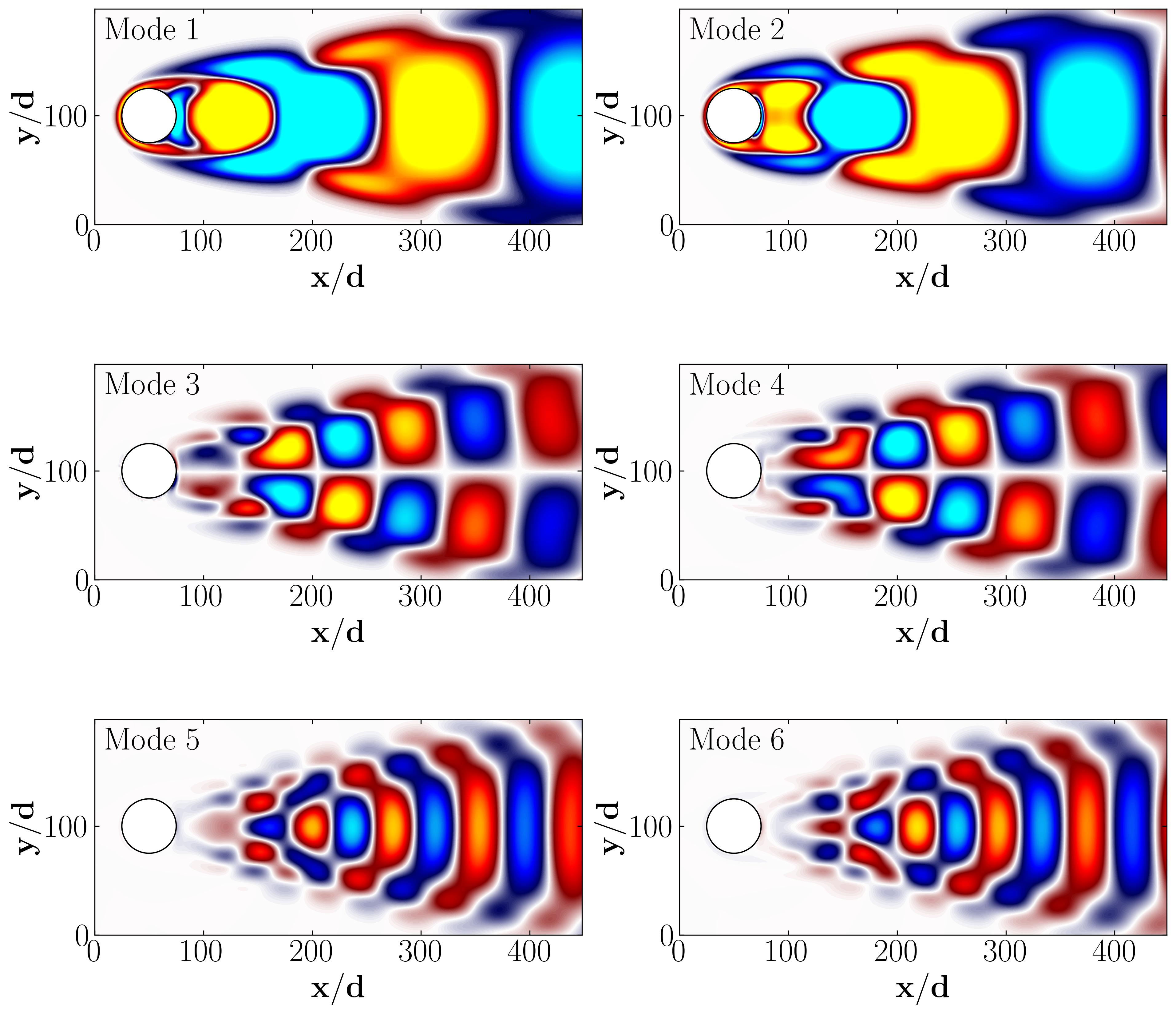
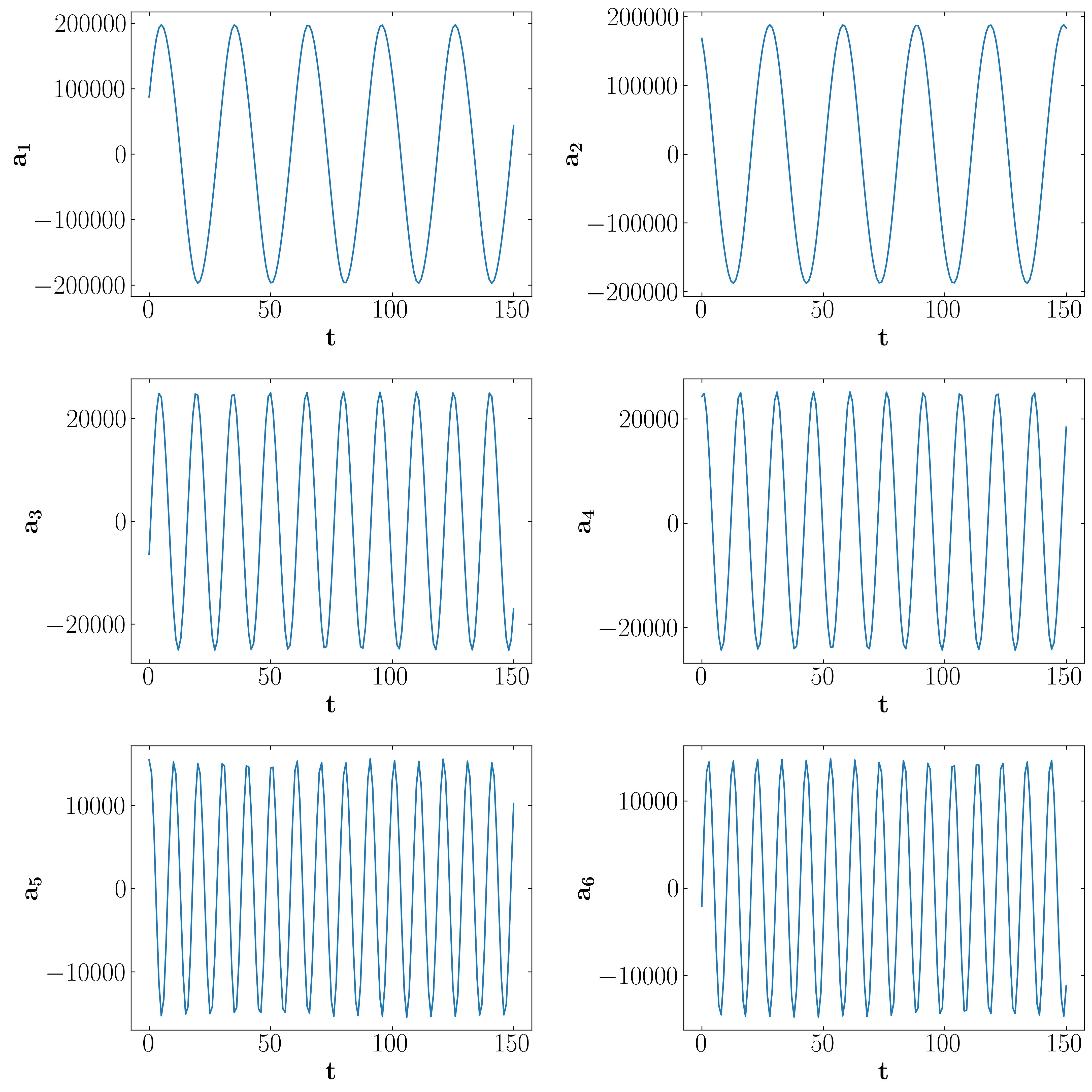
Then, you can proceed to plot the POD modes and their corresponding amplitudes as follows:

fig, axs = plt.subplots(3, 2, figsize=(15, 15))

ax = axs[0,0]
Mode = 0
p = ax.contourf(np.reshape(Phi[:,Mode],(n,m)).T, levels = 1001, vmin=-5, vmax=5, cmap = cmap.reversed())
Circle = plt.Circle((50, 100), 25, ec='k', color='white', zorder=2)
ax.add_patch(Circle)
ax.xaxis.set_tick_params(direction='in', which='both')
ax.yaxis.set_tick_params(direction='in', which='both')
ax.xaxis.set_ticks_position('both')
ax.yaxis.set_ticks_position('both')
ax.set_aspect('equal')

ax.set_xlabel(r'$\bf x/d$')
ax.set_ylabel(r'$\bf y/d$')
ax.text(10, 170, 'Mode 1', fontsize = 25, color = 'black')

ax = axs[0,1]
Mode = 1
p = ax.contourf(np.reshape(Phi[:,Mode],(n,m)).T, levels = 1001, vmin=-5, vmax=5, cmap = cmap.reversed())
Circle = plt.Circle((50, 100), 25, ec='k', color='white', zorder=2)
ax.add_patch(Circle)
ax.xaxis.set_tick_params(direction='in', which='both')
ax.yaxis.set_tick_params(direction='in', which='both')
ax.xaxis.set_ticks_position('both')
ax.yaxis.set_ticks_position('both')
ax.set_aspect('equal')

ax.set_xlabel(r'$\bf x/d$')
ax.set_ylabel(r'$\bf y/d$')
ax.text(10, 170, 'Mode 2', fontsize = 25, color = 'black')

ax = axs[1,0]
Mode = 2
p = ax.contourf(np.reshape(Phi[:,Mode],(n,m)).T, levels = 1001, vmin=-5, vmax=5, cmap = cmap.reversed())
Circle = plt.Circle((50, 100), 25, ec='k', color='white', zorder=2)
ax.add_patch(Circle)
ax.xaxis.set_tick_params(direction='in', which='both')
ax.yaxis.set_tick_params(direction='in', which='both')
ax.xaxis.set_ticks_position('both')
ax.yaxis.set_ticks_position('both')
ax.set_aspect('equal')

ax.set_xlabel(r'$\bf x/d$')
ax.set_ylabel(r'$\bf y/d$')
ax.text(10, 170, 'Mode 3', fontsize = 25, color = 'black')

ax = axs[1,1]
Mode = 3
p = ax.contourf(np.reshape(Phi[:,Mode],(n,m)).T, levels = 1001, vmin=-5, vmax=5, cmap = cmap.reversed())
Circle = plt.Circle((50, 100), 25, ec='k', color='white', zorder=2)
ax.add_patch(Circle)
ax.xaxis.set_tick_params(direction='in', which='both')
ax.yaxis.set_tick_params(direction='in', which='both')
ax.xaxis.set_ticks_position('both')
ax.yaxis.set_ticks_position('both')
ax.set_aspect('equal')

ax.set_xlabel(r'$\bf x/d$')
ax.set_ylabel(r'$\bf y/d$')
ax.text(10, 170, 'Mode 4', fontsize = 25, color = 'black')

ax = axs[2,0]
Mode = 4
p = ax.contourf(np.reshape(Phi[:,Mode],(n,m)).T, levels = 1001, vmin=-5, vmax=5, cmap = cmap.reversed())
Circle = plt.Circle((50, 100), 25, ec='k', color='white', zorder=2)
ax.add_patch(Circle)
ax.xaxis.set_tick_params(direction='in', which='both')
ax.yaxis.set_tick_params(direction='in', which='both')
ax.xaxis.set_ticks_position('both')
ax.yaxis.set_ticks_position('both')
ax.set_aspect('equal')

ax.set_xlabel(r'$\bf x/d$')
ax.set_ylabel(r'$\bf y/d$')
ax.text(10, 170, 'Mode 5', fontsize = 25, color = 'black')

ax = axs[2,1]
Mode = 5
p = ax.contourf(np.reshape(Phi[:,Mode],(n,m)).T, levels = 1001, vmin=-5, vmax=5, cmap = cmap.reversed())
Circle = plt.Circle((50, 100), 25, ec='k', color='white', zorder=2)
ax.add_patch(Circle)
ax.xaxis.set_tick_params(direction='in', which='both')
ax.yaxis.set_tick_params(direction='in', which='both')
ax.xaxis.set_ticks_position('both')
ax.yaxis.set_ticks_position('both')
ax.set_aspect('equal')

ax.set_xlabel(r'$\bf x/d$')
ax.set_ylabel(r'$\bf y/d$')
ax.text(10, 170, 'Mode 6', fontsize = 25, color = 'black')

fig.subplots_adjust(hspace=0)

plt.show()

fig, axs = plt.subplots(3, 2, figsize=(15, 15))

ax = axs[0,0]
Mode = 0
ax.plot(a[Mode,:])
ax.xaxis.set_tick_params(direction='in', which='both')
ax.yaxis.set_tick_params(direction='in', which='both')
ax.xaxis.set_ticks_position('both')
ax.yaxis.set_ticks_position('both')

ax.set_xlabel(r'$\bf t$')
ax.set_ylabel(r'$\bf a_1$')

ax = axs[0,1]
Mode = 1
ax.plot(a[Mode,:])
ax.xaxis.set_tick_params(direction='in', which='both')
ax.yaxis.set_tick_params(direction='in', which='both')
ax.xaxis.set_ticks_position('both')
ax.yaxis.set_ticks_position('both')

ax.set_xlabel(r'$\bf t$')
ax.set_ylabel(r'$\bf a_2$')

ax = axs[1,0]
Mode = 2
ax.plot(a[Mode,:])
ax.xaxis.set_tick_params(direction='in', which='both')
ax.yaxis.set_tick_params(direction='in', which='both')
ax.xaxis.set_ticks_position('both')
ax.yaxis.set_ticks_position('both')

ax.set_xlabel(r'$\bf t$')
ax.set_ylabel(r'$\bf a_3$')

ax = axs[1,1]
Mode = 3
ax.plot(a[Mode,:])
ax.xaxis.set_tick_params(direction='in', which='both')
ax.yaxis.set_tick_params(direction='in', which='both')
ax.xaxis.set_ticks_position('both')
ax.yaxis.set_ticks_position('both')

ax.set_xlabel(r'$\bf t$')
ax.set_ylabel(r'$\bf a_4$')

ax = axs[2,0]
Mode = 4
ax.plot(a[Mode,:])
ax.xaxis.set_tick_params(direction='in', which='both')
ax.yaxis.set_tick_params(direction='in', which='both')
ax.xaxis.set_ticks_position('both')
ax.yaxis.set_ticks_position('both')

ax.set_xlabel(r'$\bf t$')
ax.set_ylabel(r'$\bf a_5$')

ax = axs[2,1]
Mode = 5
ax.plot(a[Mode,:])
ax.xaxis.set_tick_params(direction='in', which='both')
ax.yaxis.set_tick_params(direction='in', which='both')
ax.xaxis.set_ticks_position('both')
ax.yaxis.set_ticks_position('both')

ax.set_xlabel(r'$\bf t$')
ax.set_ylabel(r'$\bf a_6$')

plt.tight_layout()

plt.show()

Flow reconstruction

Modal decomposition methods like POD yield modes not as functions of time, but rather as linear combinations of coefficients, as demonstrated earlier. Therefore, one can utilize the POD modes to reconstruct the flow field at any specific time instance. However, the decision on how many modes to select depends on truncating the linear combination. Thus, it’s crucial to provide a quantitative summary of the information contained in each mode. This facilitates the identification of modes with lower information content, which can be omitted. This process leads to achieving a reduced representation of the dataset, known as a reduced order model.

The amount of information represented by each POD mode is quantified within the matrix Σ or S, which contains the singular values associated with each mode. Consequently, higher singular values signify more energetic POD modes, indicating a greater amount of information from the dataset. By plotting the energy content of each mode and the cumulative energy, similar to methods used with SVD, one can assess the significance of each mode and determine the appropriate level of truncation.

Energy = np.zeros((len(S),1))
for i in np.arange(0,len(S)):
    Energy[i] = S[i]/np.sum(S)

X_Axis = np.arange(Energy.shape[0])
heights = Energy[:,0]

fig, axes = plt.subplots(1, 2, figsize = (12,4))
ax = axes[0]
ax.bar(X_Axis, heights, width=0.5)
ax.set_xlim(-0.25, 25)
ax.set_xlabel('Modes')
ax.set_ylabel('Energy Content')

ax = axes[1]
cumulative = np.cumsum(S)/np.sum(S)
ax.plot(cumulative, marker = 'o', markerfacecolor = 'none', markeredgecolor = 'k', ls='-', color = 'k')
ax.set_xlabel('Modes')
ax.set_ylabel('Cumulative Energy')
ax.set_xlim(0, 25)

plt.show()

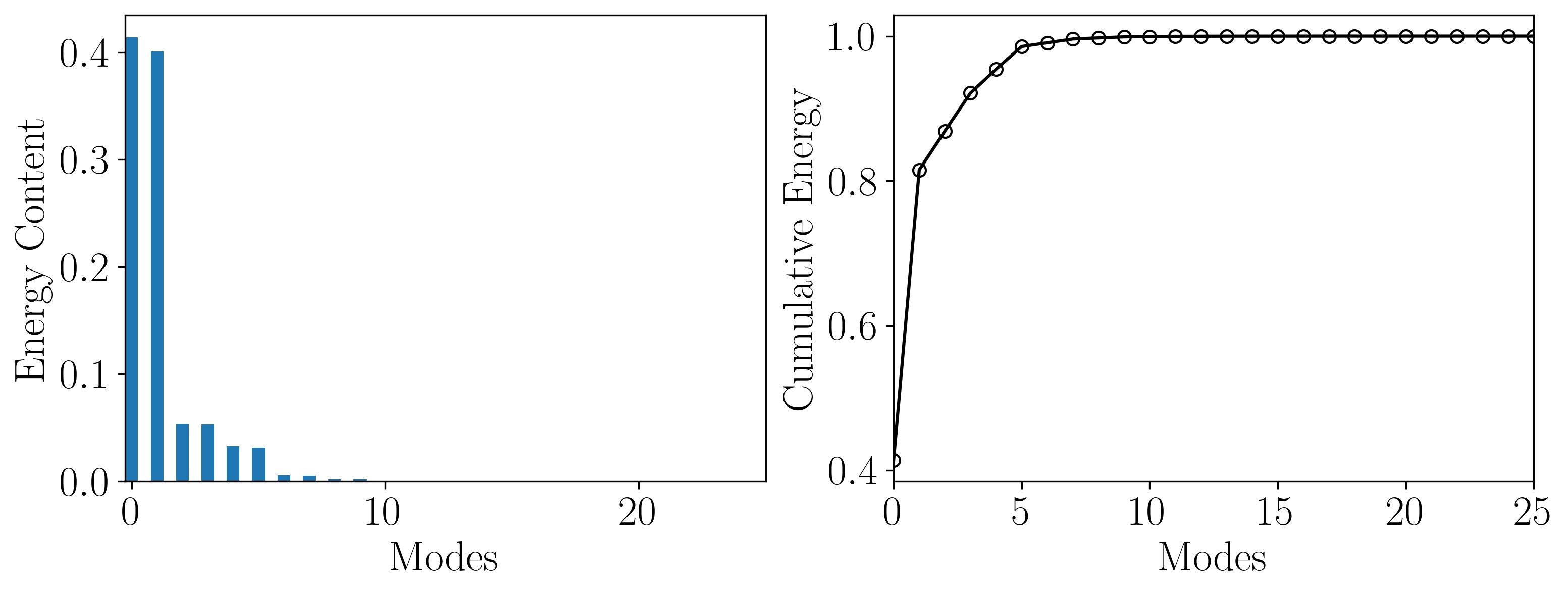
This plot demonstrates that the first 10 POD modes encapsulate nearly 99% of the total energy. Hence, one can effectively represent the flow field using only these first 10 modes. To verify this, we can attempt to reconstruct the mean-removed (fluctuating) flow field using solely the first 10 modes. Then, we’ll compare it with the original fluctuating field by:

fig, axs = plt.subplots(1, 2, figsize=(15, 15))

ax = axs[0]
p = ax.contourf(np.reshape(Y[:,0],(n,m)).T, levels = 1001, vmin=-5, vmax=5, cmap = cmap.reversed())
Circle = plt.Circle((50, 100), 25, ec='k', color='white', zorder=2)
ax.add_patch(Circle)
ax.xaxis.set_tick_params(direction='in', which='both')
ax.yaxis.set_tick_params(direction='in', which='both')
ax.xaxis.set_ticks_position('both')
ax.yaxis.set_ticks_position('both')
ax.set_aspect('equal')

ax.set_xlabel(r'$\bf x/d$')
ax.set_ylabel(r'$\bf y/d$')
ax.set_title(r'$u^\prime$(original)')
# ax.text(10, 210, r'$u^\prime$(original)', fontsize = 21, color = 'black')

ax = axs[1]
nModes = 10
sum = np.sum(Phi[:,:nModes], axis = 1)
p = ax.contourf(np.reshape(sum[:,],(n,m)).T, levels = 1001, vmin=-70, vmax=70, cmap = cmap.reversed())
Circle = plt.Circle((50, 100), 25, ec='k', color='white', zorder=2)
ax.add_patch(Circle)
ax.xaxis.set_tick_params(direction='in', which='both')
ax.yaxis.set_tick_params(direction='in', which='both')
ax.xaxis.set_ticks_position('both')
ax.yaxis.set_ticks_position('both')
ax.set_aspect('equal')

ax.set_xlabel(r'$\bf x/d$')
ax.set_ylabel(r'$\bf y/d$')
ax.set_title(r'$u^\prime$(Reconstructed using 10 modes)')

plt.show()

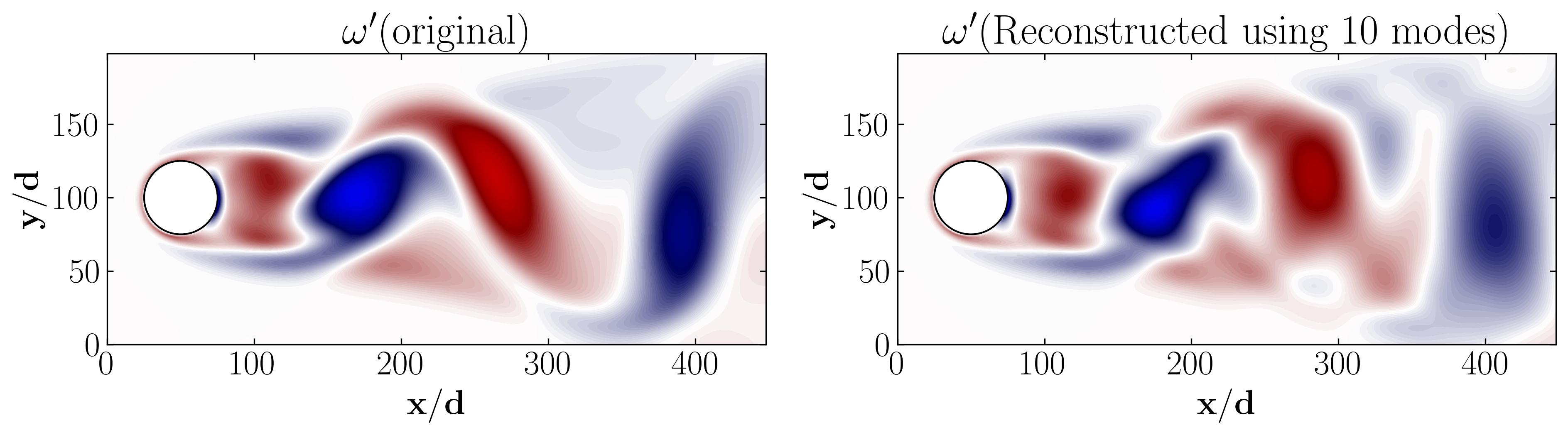
This figure essentially illustrates that the combination of the first 10 POD modes closely resembles the original fluctuating flow field. Within it, the majority of coherent flow structures are distinctly visible. This offers a simplified representation of a reduced order model, effectively capturing the essential dynamics of the system while significantly reducing computational complexity.

As we conclude this exploration, stay tuned for my upcoming articles, where I delve deeper into the practical implementation of POD using OpenFOAM simulation data. In these forthcoming articles, we’ll explore two distinct methods of performing POD using data extracted out of OpenFOAM, unlocking even greater insights into the fascinating world of fluid dynamics and computational fluid mechanics.