Get ready to explore the mathematical machinery behind Dynamic Mode Decomposition (DMD)! This article delves into the elegant formulations and algorithms that fuel this data-driven powerhouse. We’ll dissect the equations that unlock DMD’s ability to extract hidden patterns from complex data. By unraveling the algorithmic core, we’ll gain a deeper understanding of how DMD transforms high-dimensional chaos into interpretable insights.

The world around us is a symphony of interactions, shaped by dynamical systems—entities that evolve over space and time. Dynamical systems encompass the analysis, prediction, and understanding of systems described by differential equations or iterative mappings, spanning classical mechanics, fluid dynamics, climate science, finance, and more. These systems, often high-dimensional and nonlinear, exhibit rich multiscale behaviors. However, beneath this complexity lies a fundamental principle: many such systems can be distilled into low-dimensional attractors characterized by spatiotemporal coherent structures. Enter Dynamic Mode Decomposition (DMD). Situated at the confluence of mathematics, physics, and data science, DMD provides a unique lens through which we can decipher the intricate dynamics of complex systems.

For a broader introduction to DMD, check out my previous article here.

In this installment, we’ll look into the mathematics and the algorithms that fuel this data-driven powerhouse. Throughout this article, I will draw insights from the book “Dynamic Mode Decomposition: Data-Driven Modeling of Complex Systems” by J. Nathan Kutz and others.

Let’s get started!

Mathematical architecture

In essence, a dynamical system is often encapsulated through ordinary differential equations, typically nonlinear in nature. Let’s consider one such system represented as follows:

Here, 𝑥 denotes a vector representing the state of the dynamical system at any given time 𝑡, while 𝜇 encompasses the system parameters, and 𝑓(∗) signifies the system dynamics. Notably, 𝑥 tends to be quite large (𝑛»1), reflecting the system’s state derived from the discretization of a partial differential equation across numerous spatial locations. A prime example of this arises in fluid dynamics simulations, where the flow field typically comprises millions of degrees of freedom at any given time instance.

Transitioning to a discrete time representation of our dynamical system, sampled at intervals of Δ𝑡, we arrive at:

In this case we can simply give the time evolution of our system as a function of x such that,

Here, 𝑘 denotes the total number of measurements in time (snapshots), with 𝑘 = 1, 2, 3, . . ., 𝑚. These measurements essentially capture the system’s state at each time instance:

Additionally, we establish an initial condition:

Taking into account the governing equation and the initial condition of the system, we can distill this problem into an initial value problem. However, given the nonlinear nature of our system, constructing a solution without resorting to numerical approximation methods is impractical. Enter the DMD framework, which adopts an equation-free perspective. In this approach, the dynamics 𝑓(𝑥,𝑡;𝜇) may remain unknown, and thus, data measurements of the system alone are utilized to approximate the dynamics and forecast the future state. Returning to the challenge of solving a nonlinear system, one can simplify the governing equation to a locally linear system:

Indeed, when considering the initial condition 𝑥(0), the problem resembles a linear equation 𝐴𝑥=𝑏, evoking a familiar solution—the eigenvalue decomposition. This analogy highlights the utility of leveraging linear methods to approximate the dynamics of nonlinear systems, a core principle that underpins the effectiveness of techniques like DMD in uncovering hidden patterns within complex data.

Here, $φ_k$ and $ω_k$ represent the eigenvectors and eigenvalues of the matrix 𝐴, respectively, while the coefficients 𝑏𝑘 denote the coordinates of 𝑥(0) in the eigenvector basis. With this approximation of 𝑥, we can delineate the discrete-time dynamics of the system, sampled at intervals of Δ𝑡, as follows:

\(x_{k+1} = Ax_k\) where,

Here, 𝐴 is referred to as a time-map, representing the system’s evolution over time. The solution of this system can be succinctly expressed in terms of the eigenvalues 𝜆𝑘 and eigenvectors 𝜙𝑘 of the discrete-time map A:

As previously stated, b represents the coefficients of the initial condition 𝑥1 in the eigenvector basis, such that $𝑥_1=Φ𝑏$. Thus, the DMD algorithm generates a low-rank eigendecomposition of matrix 𝐴, which best fits the measured data 𝑥𝑘 for 𝑘= 1, 2, . . . , 𝑚 in a least-squares sense. This is expressed as:

The DMD algorithm minimizes the least-square approximation across all points for 𝑘= 1, 2, . . . , 𝑚−1. It’s important to note that the optimality of the approximation is confined to the sampling window where 𝐴 is constructed. However, the approximate solution isn’t limited to making future state predictions alone; it also enables the decomposition of dynamics into various time scales, given that the 𝜆𝑘 values are predetermined.

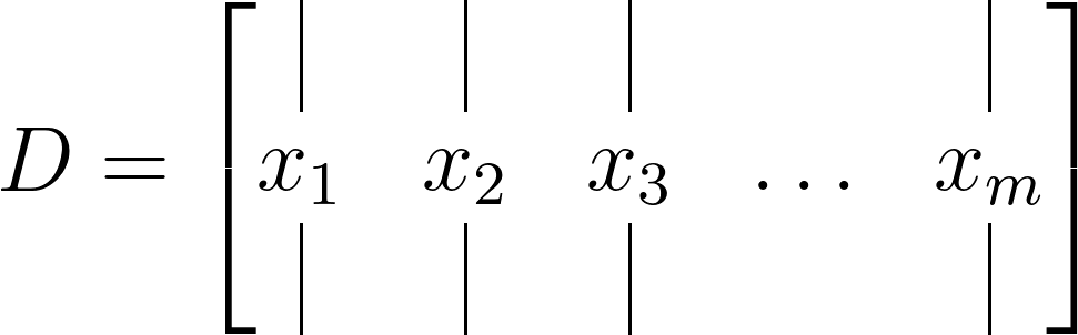
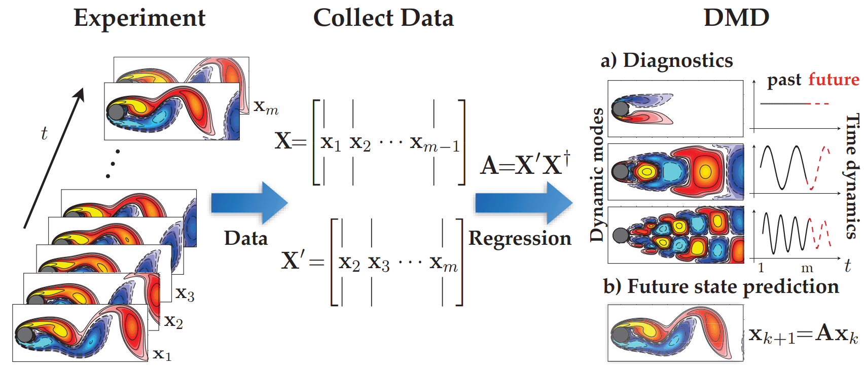
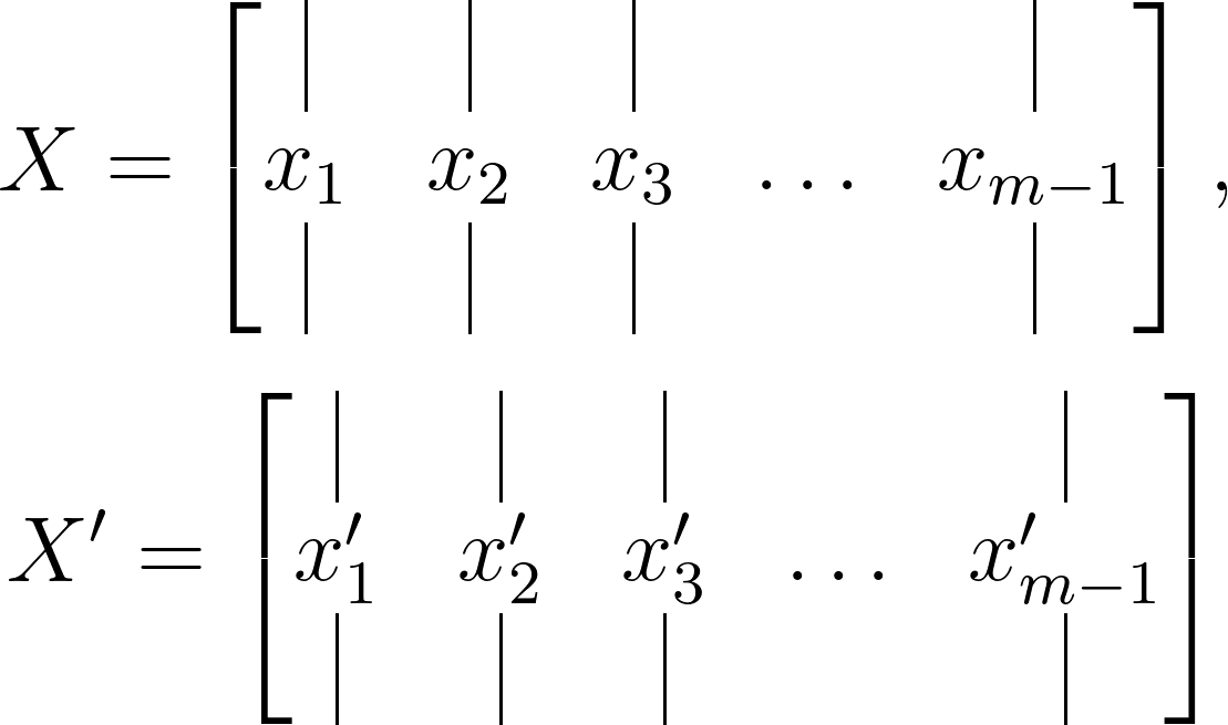
Now, let’s address the origin of this 𝑚−1. To minimize the approximation error in the least-squares method across the total number of snapshots (𝑘= 1, 2, . . . , 𝑚), the m snapshots can be organized into two large data matrices, each containing 𝑚−1 snapshots. Additionally, one data matrix is time-shifted by Δ𝑡. For instance, consider the data matrix 𝐷 defined as:

This matrix is divided into two time-shifted matrices, given as:

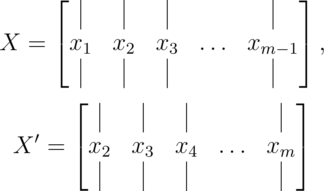
Let’s apply the analogy we developed earlier to these matrices. Firstly, remember that these data snapshots are typically sampled from a nonlinear dynamical system, like a fluid dynamics simulation or financial market outputs. Thus, drawing on our previous analogy, we aim to find an optimal local linear approximation, expressed in terms of these matrices as:

Hence, the optimal discrete-time mapping matrix 𝐴 can be expressed as:

where † denotes the Moore–Penrose pseudoinverse. This solution minimizes the error:

where ∥⋅∥𝐹 represents the Frobenius norm. Specifically, if ∥⋅∥𝐹=2 , this simplifies to an L2 least-squares approximation.

Dynamic Mode Decomposition

Building upon the mathematical framework outlined above, the modern definition of DMD, as articulated by Tu et al. (2014), can be summarized as follows:

Consider a dynamical system and two sets of data such that:

such that the temporal evolution of the system over Δ𝑡 time can be expressed by a mapping such that:

DMD computes the leading eigendecomposition of the best-fit linear mapping operator 𝐴 relating the data matrices:

such that:

The DMD modes, also referred to as dynamic modes, are the eigenvectors of 𝐴, and each DMD mode corresponds to a particular eigenvalue of 𝐴.

The DMD method offers a spatio-temporal decomposition of data into dynamic modes derived from snapshots or measurements of a system over time. The mathematical principles behind extracting dynamic information from time-resolved snapshots share a kinship with the Arnoldi algorithm, a stalwart of fast computational solvers. The data collection process involves two parameters: 𝑛, specifying the spatial degrees of freedom per snapshot, and 𝑚, denoting the number of snapshots taken.

It is important to note that DMD may be though of as a linear regression of data into the dynamics given by A. However, there are some key differences between the two. Most prominently, we are assuming that the snapshots xk in our data matrix X are high dimensional so that the matrix is tall and skinny, meaning that the size n of a snapshot is larger than the number m −1 of snapshots. To provide perspective, assume that n is equal to 1 Billion, thus A then will have 1 Billion elements and may become too unweildy to represent or even decompose. However, if the rank of A is at most m-1, equal to the number of snapshots, since it is constructed as a linear combination of the m − 1 columns of X′. In this case, instead of solving for A directly, we first project our data onto a low-rank subspace defined by at most m − 1 POD modes and then solve for a low-dimensional evolution $\tilde{A}$ that evolves on these POD mode coefficients. The DMD algorithm then uses this low-dimensional operator $\tilde{A}$ to reconstruct the leading nonzero eigenvalues and eigenvectors of the fulldimensional operator A without ever explicitly computing A.

It’s crucial to recognize that while DMD can be conceptualized as a linear regression of data into the dynamics given by 𝐴, there exist significant differences between the two. Notably, we assume that the snapshots 𝑥𝑘 in our data matrix 𝑋 are high-dimensional, resulting in a tall and skinny matrix. This means that the size 𝑛 of a snapshot surpasses the number 𝑚−1 of snapshots. To illustrate, envision 𝑛 equating to 1 billion, rendering 𝐴 unwieldy to represent or decompose. However, if the rank of 𝐴 is at most 𝑚−1, mirroring the number of snapshots, since it’s constructed as a linear combination of the 𝑚−1 columns of 𝑋, we first project our data onto a low-rank subspace defined by at most 𝑚−1 POD modes. Then, we solve for a low-dimensional evolution $\tilde{A}$ that operates on these POD mode coefficients. Subsequently, the DMD algorithm employs this low-dimensional operator $\tilde{A}$ to reconstruct the leading nonzero eigenvalues and eigenvectors of the full-dimensional operator 𝐴 without explicitly computing.

Koopman operator

The Dynamic Mode Decomposition method approximates the modes of the Koopman operator. This operator is a linear, infinite-dimensional entity that illustrates how a nonlinear dynamical system acts on the Hilbert space of measurement functions of the state. Let’s simplify this concept.

Imagine you have a magical machine that can predict the future movements of a bouncing ball. You feed information about the ball’s position and velocity into the machine, and out comes a prediction of where the ball will be in the next few seconds. Now, let’s break down how this magical machine works using the idea of the Koopman operator:

• Observables: The information you feed into the machine, like the position and velocity of the ball, are what we call observables. These are the things we can measure or observe about the system.
• State space: Think of the state space as the “world” in which the ball exists. It’s like a big playground where the ball can bounce around freely. The state space includes all possible positions and velocities the ball could have.
• Koopman operator: Now, imagine the magical machine as the Koopman operator. It’s like a super smart mathematician that takes the observables you give it (the ball’s position and velocity) and performs some fancy calculations to predict the future behavior of the system. It does this by transforming observables from one state to another, sort of like predicting where the ball will be based on its current position and velocity.

So, in essence, the Koopman operator is like a magical machine that operates on observables in the state space to predict future behavior.

It’s crucial to recognize that the Koopman operator doesn’t rely on linearization of dynamics; rather, it portrays the flow of a dynamical system on measurement functions as an infinite-dimensional operator. The DMD method can be perceived as computing, from experimental or numerical data, the eigenvalues and eigenvectors (low-dimensional modes) of a finite-dimensional linear model approximating the infinite-dimensional Koopman operator. Given the linearity of the operator, this decomposition reveals the growth rates and frequencies associated with each mode.

Mathematically, the Koopman operator (𝐾) is an infinite-dimensional linear operator acting on the Hilbert space (𝐻) comprising all scalar-valued measurements of the state (𝑔(𝑥)). The Koopman operator’s action on the measurement function 𝑔 is represented as:

This implies that:

In essence, the Koopman operator advances measurements alongside the flow 𝐹, showcasing its robustness and generality, as it applies to all measurement functions 𝑔 evaluated at any state vector 𝑥. Approximating the Koopman operator forms the crux of the DMD methodology, as the mapping over Δ𝑡 is linear, even though the underlying dynamics $𝑥_𝑘$ may be nonlinear.

In summary, Dynamic Mode Decomposition resembles a locally linear regression of data. In this article, we’ve delved into the mathematical framework behind DMD and explored the various intricate concepts governing its methodology. In the next installment, I’ll elucidate the general DMD algorithm and provide a toy example to better illustrate the concept of understanding a dynamic system using DMD.