Dynamic Mode Decomposition using OpenFOAM and Python
Unraveling the mysteries of fluid flow just got easier! This article explores the powerful combination of Python scripting and Dynamic Mode Decomposition (DMD). We’ll leverage Python’s capabilities to compute DMD on 2D slice data extracted from OpenFOAM simulations. By harnessing this approach, we can extract hidden patterns and gain deeper insights into fluid dynamics phenomena.
Using the open-source CFD powerhouse OpenFOAM, there are two methods for computing DMD with your CFD data. The first method involves reading OpenFOAM fields directly into Python, while the second method focuses on extracting 2D slices from OpenFOAM and then computing the DMD using that data. In my previous article, I explored the first method of computing Dynamic Mode Decomposition.
In this article, we will leverage Python’s powerful libraries to directly analyze 2D slice data extracted from OpenFOAM, performing DMD and visualizing the extracted modes.
Lets begin!!!
Setting Up the Case
In this article we are analyzing the two-dimensional flow around a square cylinder at a Reynolds number of 100. This configuration closely adheres to the guidelines laid out by Bai and Alam (2018) for reference, ensuring a robust methodology. Detailed instructions for this setup are available in their work, providing invaluable guidance for alignment. A comprehensive guide to prepping your OpenFOAM case for Modal Decompositions is available here, offering detailed insights into the necessary steps.
Our journey begins with a fully-developed, statistically steady flow around a square cylinder at a Reynolds number of 100, as discussed in our previous article. Here, we extend our analysis by running this case for an additional 100 vortex shedding cycles. Within each shedding cycle, we extract two-dimensional slices or surfaces from the data 16 times. The extraction of 2D slices is facilitated by utilizing the surfaces function object in OpenFOAM, as illustrated below:
surfaces
{
    type            surfaces;
    libs            ("libsampling.so");
    writeControl   	timeStep;
    writeInterval   142;

    surfaceFormat   vtk;
    fields          (p U);

    interpolationScheme cellPoint;

    surfaces
    {
        zNormal
        {
            type        cuttingPlane;
            point       (0 0 0.05);
            normal      (0 0 1);
            interpolate true;
        }
    };
};
// ************************************************************************* //
Once the simulation run is complete, you should find a directory named surfaces within the postProcessing directory of your case, containing all the extracted surfaces.
surfaces/
├── 4771.2000000577236
│   └── zNormal.vtp
├── 4772.6200000577546
│   └── zNormal.vtp
├── 4774.0400000577856
│   └── zNormal.vtp
├── 4775.4600000578166
│   └── zNormal.vtp
.
.
.
Ensure that both the case and the surfaces are extracted before proceeding further.
Extracting data from surfaces
To extract data from the VTK files obtained from the OpenFOAM case, we will utilize PyVista. PyVista serves as a helper module for the Visualization Toolkit (VTK), wrapping the VTK library through NumPy and allowing direct array access via various methods and classes. This package offers a Pythonic, well-documented interface that exposes VTK’s robust visualization backend, facilitating rapid prototyping, analysis, and visual integration of spatially referenced datasets.
PyVista proves invaluable for scientific plotting in presentations and research papers, serving also as a supporting module for other Python modules dependent on mesh 3D rendering.
Begin by opening up a Jupyter notebook and importing the necessary modules, including PyVista:
import matplotlib.colors
import matplotlib.pyplot as plt
import numpy as np
import pandas as pd
import fluidfoam as fl
import scipy as sp
import os
import matplotlib.animation as animation
import pyvista as pv
import imageio
import io
%matplotlib inline
plt.rcParams.update({'font.size' : 18, 'font.family' : 'Times New Roman', "text.usetex": True})
Setting Path Variables and Constants:
### Constants
d = 0.1
Ub = 0.015

### Paths
Path = 'E:/Blog_Posts/Simulations/Sq_Cyl_Surfaces/surfaces/'
save_path = 'E:/Blog_Posts/SquareCylinderData/'

Files = os.listdir(Path)
Now, let’s attempt to read the first snapshot surface using PyVista:
Data = pv.read(Path + Files[0] + '/zNormal.vtp')
grid = Data.points
x = grid[:,0]
y = grid[:,1]
z = grid[:,2]
rows, columns = np.shape(grid)
print('rows = ', rows, 'columns = ', columns)

print(Data.array_names)
Output:
['TimeValue', 'p', 'U']
Here, we observe that our 2D slices encompass velocity and pressure fields. Leveraging PyVista, we can extract the vorticity field for each snapshot and organize the resulting data into a large, tall, and slender matrix to facilitate POD computation.
Data = pv.read(Path + Files[0] + '/zNormal.vtp')
grid = Data.points
x = grid[:,0]
y = grid[:,1]
z = grid[:,2]
rows, columns = np.shape(grid)
print('rows = ', rows, 'columns = ', columns)

### For U
Snaps = len(Files) # Number of snapshots
data_Vort = np.zeros((rows,Snaps-1))
for i in np.arange(0,Snaps-1):
    data = pv.read(Path + Files[i] + '/zNormal.vtp')
    gradData = data.compute_derivative('U', vorticity=True)
    grad_pyvis = gradData.point_data['vorticity']
    data_Vort[:,i:i+1] = np.reshape(grad_pyvis[:,2], (rows,1), order='F')

np.save(save_path + 'VortZ.npy', data_Vort)
Let’s examine the size of the matrix we’re dealing with by querying the shape of the data_Vort array:
data_Vort.shape
### OUTPUT
### (96624, 1600)
Additionally, we can visualize a snapshot of the vorticity field:
Proper Orthogonal Decomposition
To determine the rank of approximation for DMD, let’s first compute Proper Orthogonal Decomposition using the vorticity field data.
### POD Analysis

### Data Matrix
X = data_Vort

### Mean-removed Matrix
X_mean = np.mean(X, axis = 1)
Y = X - X_mean[:,np.newaxis]

### Covariance Matrix
C = np.dot(Y.T, Y)/(Y.shape[1]-1)

### SVD of Covariance Matrix
U, S, V = np.linalg.svd(C)

### POD modes
Phi_POD = np.dot(Y, U)

### Temporal coefficients
a = np.dot(Phi_POD.T, Y)
Using the POD eigenvalues, let’s investigate the energy content of the modes:
Energy = np.zeros((len(S),1))
for i in np.arange(0,len(S)):
    Energy[i] = S[i]/np.sum(S)

X_Axis = np.arange(Energy.shape[0])
heights = Energy[:,0]

fig, axes = plt.subplots(1, 2, figsize = (12,4))
ax = axes[0]
ax.plot(Energy, marker = 'o', markerfacecolor = 'none', markeredgecolor = 'k', ls='-', color = 'k')
ax.set_xlim(0, 20)
ax.set_xlabel('Modes')
ax.set_ylabel('Energy Content')

ax = axes[1]
cumulative = np.cumsum(S)/np.sum(S)
ax.plot(cumulative, marker = 'o', markerfacecolor = 'none', markeredgecolor = 'k', ls='-', color = 'k')
ax.set_xlabel('Modes')
ax.set_ylabel('Cumulative Energy')
ax.set_xlim(0, 20)

plt.show()
Here, the first 21 POD modes encompass nearly 99.9% of the total energy, so using a rank-21 approximation for DMD will suffice.
Here are the POD modes for reference:
Dynamic Mode Decomposition
We will use the following function to compute DMD:
def DMD(X1, X2, r, dt):
    U, s, Vh = np.linalg.svd(X1, full_matrices=False)
    ### Truncate the SVD matrices
    Ur = U[:, :r]
    Sr = np.diag(s[:r])
    Vr = Vh.conj().T[:, :r]

    ### Build the Atilde and find the eigenvalues and eigenvectors
    Atilde = Ur.conj().T @ X2 @ Vr @ np.linalg.inv(Sr)
    Lambda, W = np.linalg.eig(Atilde)

    ### Compute the DMD modes
    Phi = X2 @ Vr @ np.linalg.inv(Sr) @ W

    omega = np.log(Lambda)/dt ### continuous time eigenvalues

    ### Compute the amplitudes

    alpha1 = np.linalg.lstsq(Phi, X1[:, 0], rcond=None)[0] ### DMD mode amplitudes

    b = np.linalg.lstsq(Phi, X2[:, 0], rcond=None)[0] ### DMD mode amplitudes

    ### DMD reconstruction
    time_dynamics = None
    for i in range(X1.shape[1]):
        v = np.array(alpha1)[:,0]*np.exp( np.array(omega)*(i+1)*dt)
        if time_dynamics is None:
            time_dynamics = v
        else:
            time_dynamics = np.vstack((time_dynamics, v))
    X_dmd = np.dot( np.array(Phi), time_dynamics.T)

    return Phi, omega, Lambda, alpha1, b, X_dmd
To use this function, let’s first obtain our time-shifted data matrices:
# get two views of the data matrix offset by one time step
X1 = np.matrix(X[:, 0:-1])
X2 = np.matrix(X[:, 1:])
And define the rank of approximation and the time-step:
r = 21
dt = 0.01*142
Then simply use the function above to compute DMD:
Phi, omega, Lambda, alpha1, b, X_dmd = DMD(X1, X2, r, dt)
Now, before diving into visualization, let’s examine the distribution of eigenvalues extracted from the DMD algorithm. Specifically, we need to understand the dynamic behavior of the DMD modes we’ve identified. To do this, plot a simple unit circle and overlay the scatter plot of the real versus imaginary eigenvalues onto it by:
theta = np.linspace( 0 , 2 * np.pi , 150 )
radius = 1
a = radius * np.cos( theta )
b = radius * np.sin( theta )

fig, ax = plt.subplots()

ax.scatter(np.real(Lambda), np.imag(Lambda), color = 'r', marker = 'o', s = 100)
ax.plot(a, b, color = 'k', ls = '--')

ax.set_xlabel(r'$\Lambda_r$')
ax.set_ylabel(r'$\Lambda_i$')

ax.set_aspect('equal')

plt.show()
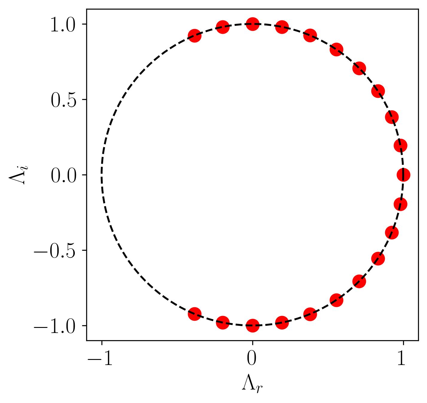
In this plot, all points lie on the unit circle, indicating that the modes neither grow nor decay, signifying stable DMD modes.
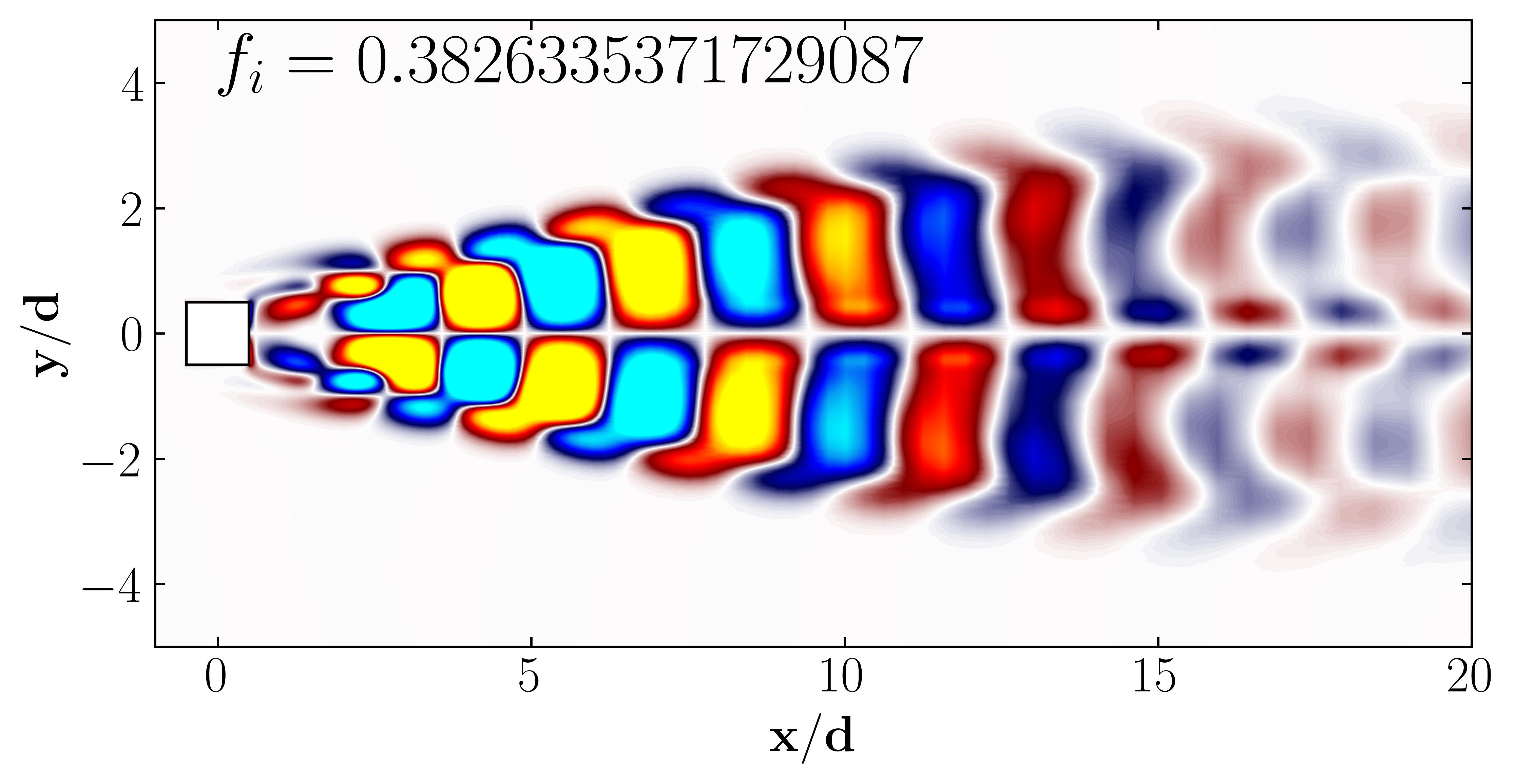
To visualize the DMD modes, first convert the DMD mode matrix into an array using the squeeze function within NumPy.
A = np.squeeze(np.asarray(Phi))
Then, simply plot the DMD modes using Matplotlib as follows:
Rect1 = plt.Rectangle((-0.5, -0.5), 1, 1, ec='k', color='white', zorder=2)
Mode = 11
fig, ax = plt.subplots(figsize=(11, 4))

p = ax.tricontourf(x/0.1, y/0.1, np.real(A[:,Mode]), levels = 1001, vmin=-0.005, vmax=0.005, cmap = cmap)

ax.add_patch(Rect1)
# ax.axvline(0.1856, c='w', ls='--', lw=1)
# ax.axvline(0.1856/2, c='w', ls='--', lw=1)
ax.xaxis.set_tick_params(direction='in', which='both')
ax.yaxis.set_tick_params(direction='in', which='both')
ax.xaxis.set_ticks_position('both')
ax.yaxis.set_ticks_position('both')
# ax.set_xscale('log')

ax.set_xlim(-1, 20)
ax.set_ylim(-5, 5)

# cb.ax.xaxis.set_ticks_position("bottom")

ax.set_aspect('equal')

ax.set_xlabel(r'$\bf x/d$')
ax.set_ylabel(r'$\bf y/d$')
# ax.set_title(r'$\bf x/d = 1$')
ax.text(0, 4, r'$f_i =' + str(np.imag(Lambda[Mode])) + '$', fontsize = 25, color = 'black')

# plt.savefig('E:/Blog_Posts/OpenFOAM/ROM_Series/Post24/Vorticity.jpeg', dpi = 600, bbox_inches = 'tight')

plt.show()
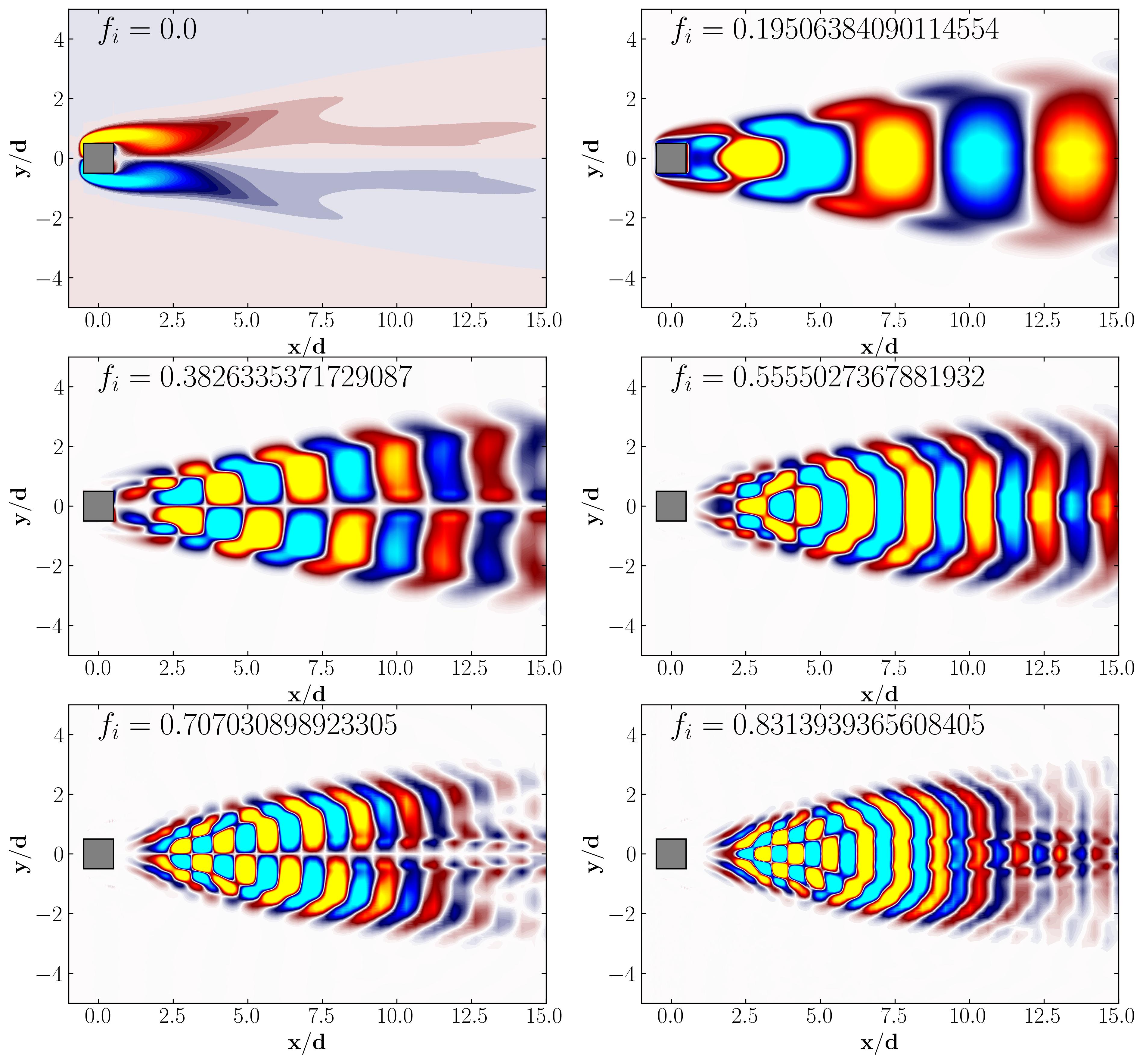
Similarly, one can plot the first 6 DMD modes as follows:
Enjoy Reading This Article?
Here are some more articles you might like to read next: