Dynamic Mode Decomposition (DMD) has revolutionized the analysis of complex systems. However, its capabilities have boundaries. This article explores two key limitations of DMD: its struggle with translational and rotational invariances, and its challenges in capturing transient phenomena. Understanding these limitations helps us choose the right tool for the job and explore alternative methods when needed.

In my previous article, I focused on the fundamental framework and basic applications of Dynamic Mode Decomposition (DMD). DMD offers a powerful method for unraveling complex spatio-temporal dynamics from data, breaking it down into dynamic modes derived from snapshots or measurements over time. Essentially, DMD is an equation-free and data-driven approach for understanding complex dynamical systems, with applications ranging from fluid dynamics to neuroscience. However, like any method, DMD has its limitations.

Similar to Principal Component Analysis (PCA), DMD relies on Singular Value Decomposition (SVD) to extract correlated patterns in the data. A key weakness of SVD-based approaches is their inefficiency in handling translational and rotational invariances in the data. Additionally, transient phenomena are not well captured by these methods.

In this article, let’s explore the weaknesses of DMD to gain a better perspective on how to use this methodology more effectively. In this article, I will draw insights from the book “Dynamic Mode Decomposition: Data-Driven Modeling of Complex Systems” by J. Nathan Kutz and others.

Lets begin!!!

Translational and Rotational Invariance

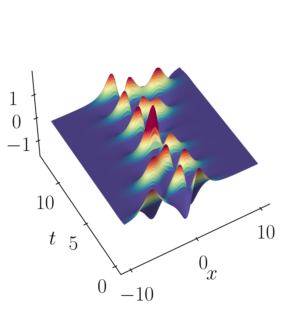
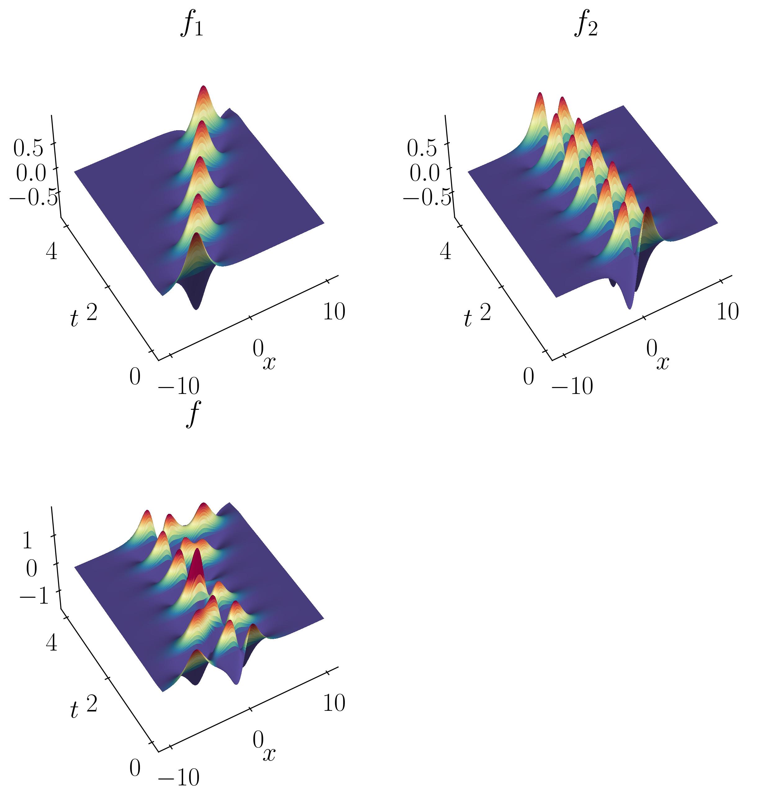
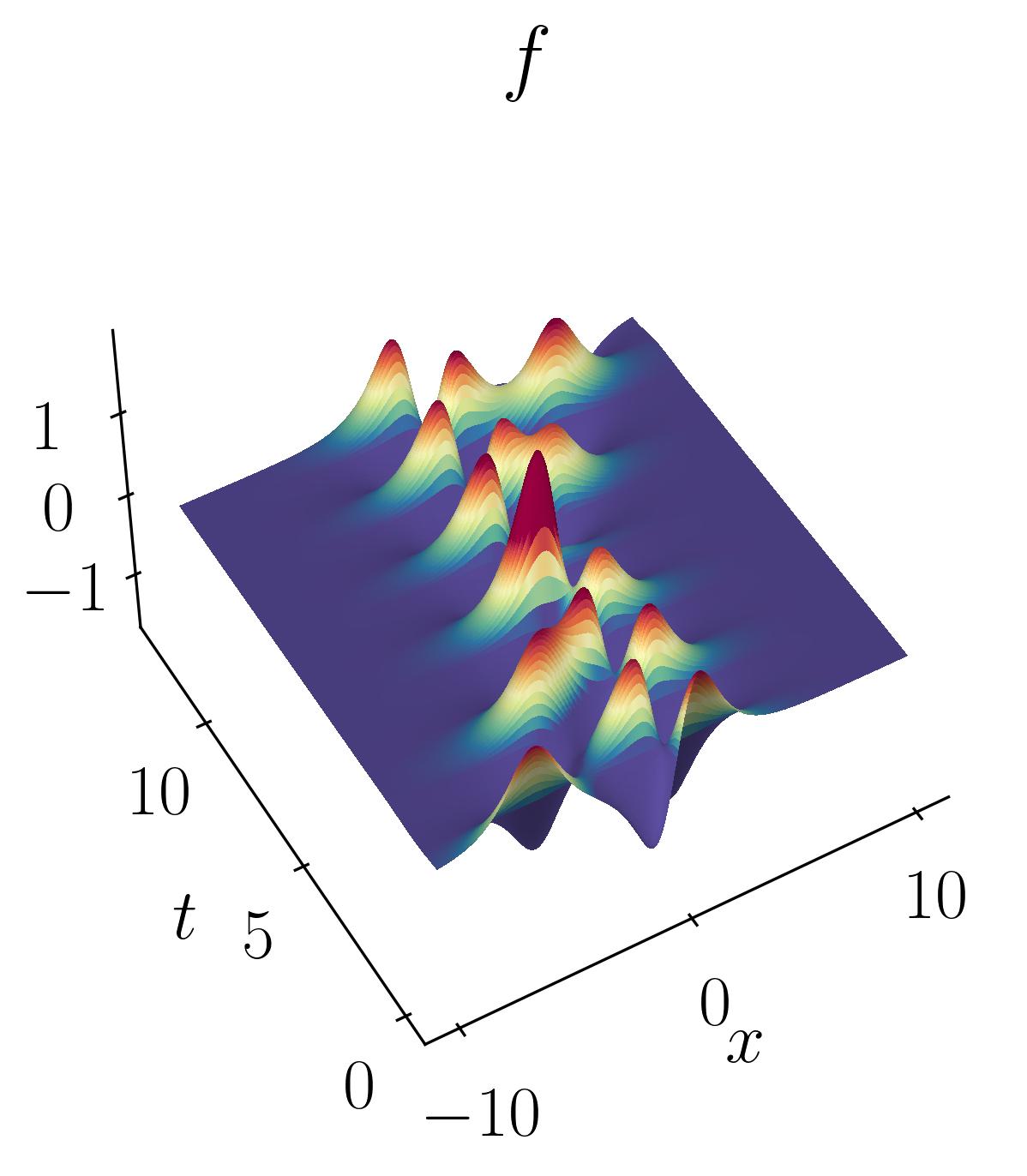
Let’s consider a toy example of two mixed spatio-temporal signals. In this case, one of the signals is translating at a constant velocity across the spatial domain. The two signals we’re considering are:

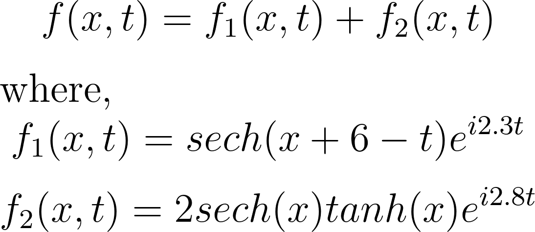
These signals have frequencies of ω1 = 2.3 and ω2 = 2.8, with distinct spatial structures:

Let’s start by opening a Jupyter notebook and importing the necessary modules:

import matplotlib.colors
import matplotlib.pyplot as plt
import numpy as np
import pandas as pd
import scipy as sp
import os
import io
import imageio
%matplotlib inline
plt.rcParams.update({'font.size' : 20, 'font.family' : 'Times New Roman', "text.usetex": True})

After that, generate the toy signals:

### Define the time and space discretization
xi = np.linspace(-10, 10, 400)
t = np.linspace(0, 4*np.pi, 200)
dt = t[1] - t[0]
[Xgrid, Tgrid] = np.meshgrid(xi, t)

### Create two spatio-temporal signals
def sech(x):
    return 1/np.cosh(x)

f1 = sech(Xgrid+6-Tgrid) * (1*np.exp(1j*2.3*Tgrid))
f2 = (sech(Xgrid)*np.tanh(Xgrid))*(2*np.exp(1j*2.8*Tgrid))

### Combine the signals
f = f1 + f2
X = f.T

Then, you can effortlessly plot the surfaces using matplotlib plotting routines like so:

fig = plt.figure(figsize=(10,10))
ax1 = fig.add_subplot(2,2,1, projection='3d')
ax1.plot_surface(Xgrid, Tgrid/np.pi, np.real(f1), 
                 #alpha = 0.7, linewidth = 0.3, edgecolor = 'black', 
                 #cmap = 'Spectral_r'
                 rstride=1, cstride=1, linewidth=0, antialiased=False, 
                 facecolors=plt.cm.Spectral_r(np.real(f1)))
ax1.set_xlabel(r'$x$')
ax1.set_ylabel(r'$t$')
# make the panes transparent
ax1.xaxis.set_pane_color((1.0, 1.0, 1.0, 0.0))
ax1.yaxis.set_pane_color((1.0, 1.0, 1.0, 0.0))
ax1.zaxis.set_pane_color((1.0, 1.0, 1.0, 0.0))
# make the grid lines transparent
ax1.xaxis._axinfo["grid"]['color'] =  (1,1,1,0)
ax1.yaxis._axinfo["grid"]['color'] =  (1,1,1,0)
ax1.zaxis._axinfo["grid"]['color'] =  (1,1,1,0)
ax1.view_init(50,240)
ax1.set_box_aspect(None, zoom=1)

ax2 = fig.add_subplot(2,2,2, projection='3d')
ax2.plot_surface(Xgrid, Tgrid/np.pi, np.real(f2), 
                 #alpha = 0.7, linewidth = 0.3, edgecolor = 'black', 
                 #cmap = 'Spectral_r'
                 rstride=1, cstride=1, linewidth=0, antialiased=False, 
                 facecolors=plt.cm.Spectral_r(np.real(f2)))
ax2.set_xlabel(r'$x$')
ax2.set_ylabel(r'$t$')
# make the panes transparent
ax2.xaxis.set_pane_color((1.0, 1.0, 1.0, 0.0))
ax2.yaxis.set_pane_color((1.0, 1.0, 1.0, 0.0))
ax2.zaxis.set_pane_color((1.0, 1.0, 1.0, 0.0))
# make the grid lines transparent
ax2.xaxis._axinfo["grid"]['color'] =  (1,1,1,0)
ax2.yaxis._axinfo["grid"]['color'] =  (1,1,1,0)
ax2.zaxis._axinfo["grid"]['color'] =  (1,1,1,0)
ax2.view_init(50,240)
ax2.set_box_aspect(None, zoom=1)

ax3 = fig.add_subplot(2,2,3, projection='3d')
ax3.plot_surface(Xgrid, Tgrid/np.pi, np.real(f), 
                 #alpha = 0.7, linewidth = 0.3, edgecolor = 'black', 
                 #cmap = 'Spectral_r'
                 rstride=1, cstride=1, linewidth=0, antialiased=False, 
                 facecolors=plt.cm.Spectral_r(np.real(f)))
ax3.set_xlabel(r'$x$')
ax3.set_ylabel(r'$t$')
# make the panes transparent
ax3.xaxis.set_pane_color((1.0, 1.0, 1.0, 0.0))
ax3.yaxis.set_pane_color((1.0, 1.0, 1.0, 0.0))
ax3.zaxis.set_pane_color((1.0, 1.0, 1.0, 0.0))
# make the grid lines transparent
ax3.xaxis._axinfo["grid"]['color'] =  (1,1,1,0)
ax3.yaxis._axinfo["grid"]['color'] =  (1,1,1,0)
ax3.zaxis._axinfo["grid"]['color'] =  (1,1,1,0)
ax3.view_init(50,240)
ax3.set_box_aspect(None, zoom=1)
fig.subplots_adjust(hspace=0)
plt.show()

Here is the DMD algorithm I will utilize:

def DMD(X1, X2, r, dt):
    U, s, Vh = np.linalg.svd(X1, full_matrices=False)
    ### Truncate the SVD matrices
    Ur = U[:, :r]
    Sr = np.diag(s[:r])
    Vr = Vh.conj().T[:, :r]
    
    ### Build the Atilde and find the eigenvalues and eigenvectors
    Atilde = Ur.conj().T @ X2 @ Vr @ np.linalg.inv(Sr)
    Lambda, W = np.linalg.eig(Atilde)
    
    ### Compute the DMD modes
    Phi = X2 @ Vr @ np.linalg.inv(Sr) @ W
    
    omega = np.log(Lambda)/dt ### continuous time eigenvalues
    
    ### Compute the amplitudes
    
    alpha1 = np.linalg.lstsq(Phi, X1[:, 0], rcond=None)[0] ### DMD mode amplitudes
    
    b = np.linalg.lstsq(Phi, X2[:, 0], rcond=None)[0] ### DMD mode amplitudes
    
    ### DMD reconstruction
    time_dynamics = None
    for i in range(X1.shape[1]):
        v = np.array(alpha1)[:,0]*np.exp( np.array(omega)*(i+1)*dt)
        if time_dynamics is None:
            time_dynamics = v
        else:
            time_dynamics = np.vstack((time_dynamics, v))
    X_dmd = np.dot( np.array(Phi), time_dynamics.T)
    
    return Phi, omega, Lambda, alpha1, b, X_dmd

At this stage, since our objective is to apply DMD to our toy dataset, let’s begin by generating the two data matrices as outlined in the DMD algorithm.

# get two views of the data matrix offset by one time step
X1 = np.matrix(X[:, 0:-1])
X2 = np.matrix(X[:, 1:])

Next, utilize the previously defined DMD function to compute rank-2, rank-5, and rank-10 reconstructions of the original signal:

Phi, omega, Lambda, alpha1, b, X_dmd = DMD(X1, X2, 2, dt)

The DMD reconstruction can then be plotted using simple matplotlib routines as shown before. Below are the comparative results of the original signal versus the rank-2, rank-5, and rank-10 DMD reconstructions:

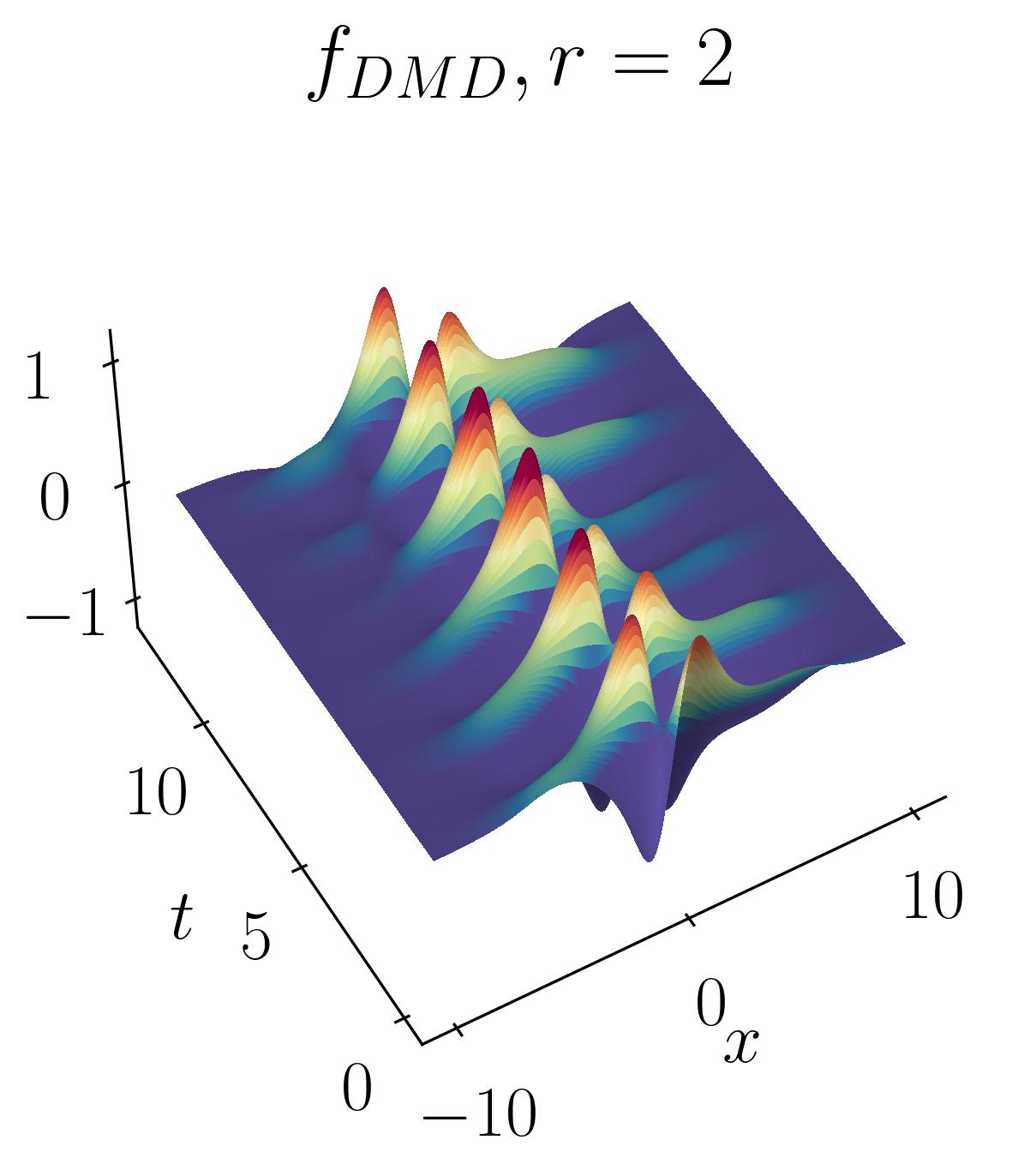
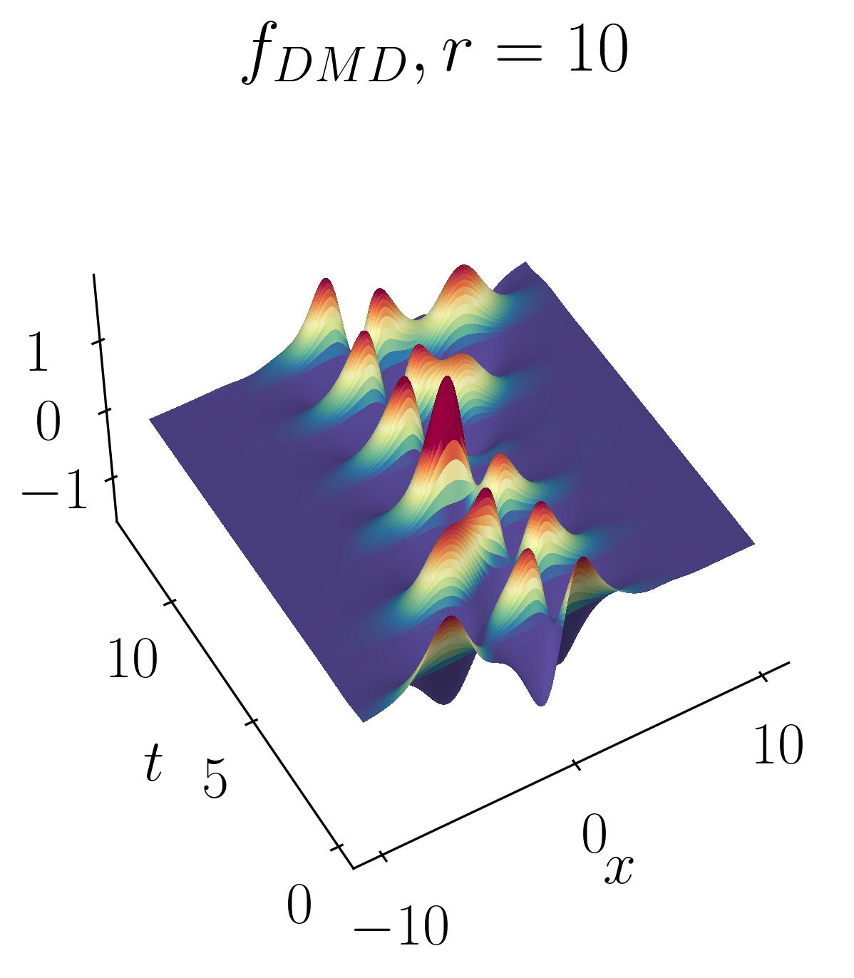
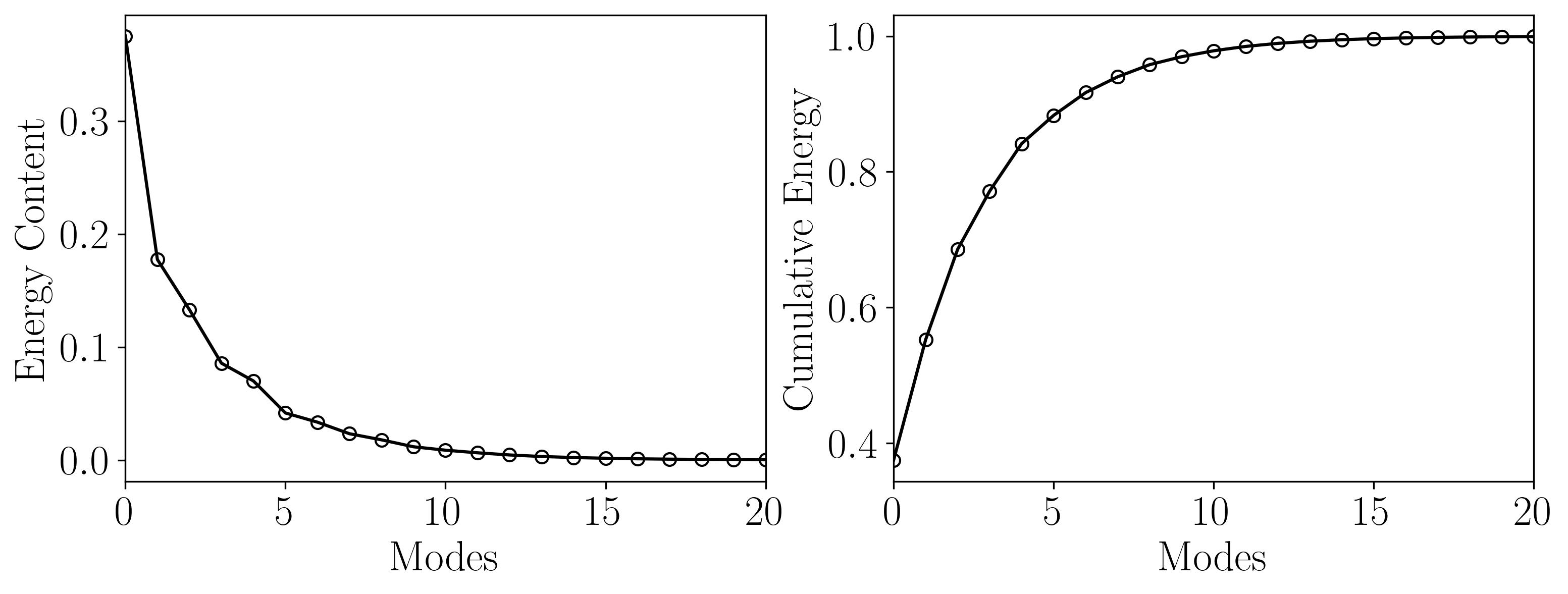
As observed, the rank-2 reconstruction is unable to accurately characterize the dynamics due to the translation. It now takes nearly 10 modes to achieve an accurate reconstruction. This artificial inflation of the dimension arises from the inability of SVD to capture translational invariances and correlate across snapshots of time. We can verify this using Singular Value Decomposition and plotting the energy content as a function of the number of modes, as shown below:

This limitation of DMD is effectively addressed using the multiresolution DMD (mrDMD) method.

Transient Phenomenon

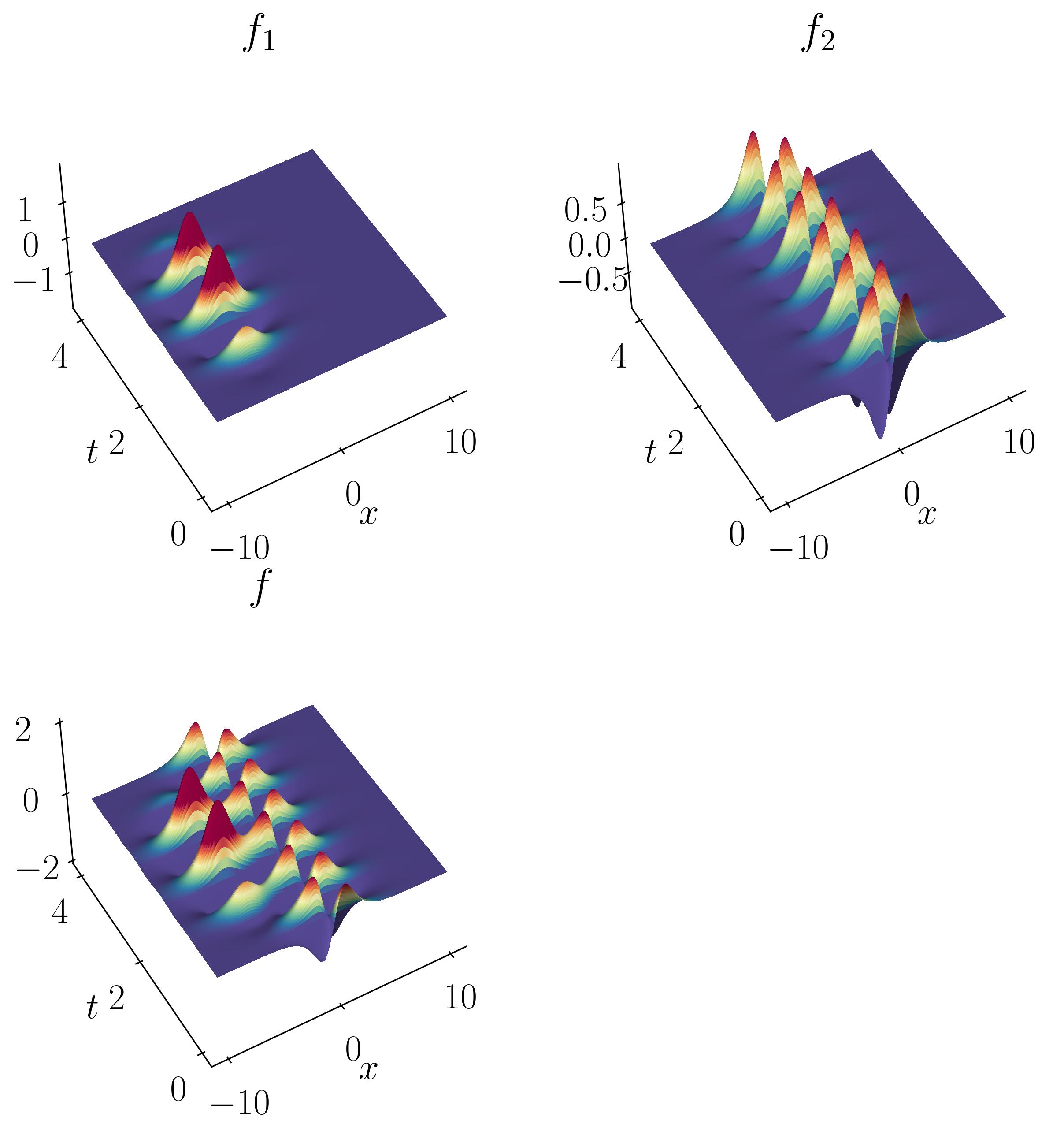
Transient phenomena are also challenging to approximate using DMD and PCA methods. To demonstrate this, let’s consider a simple example of two mixed spatio-temporal signals, with one turning on and off temporally. The signals we are examining are:

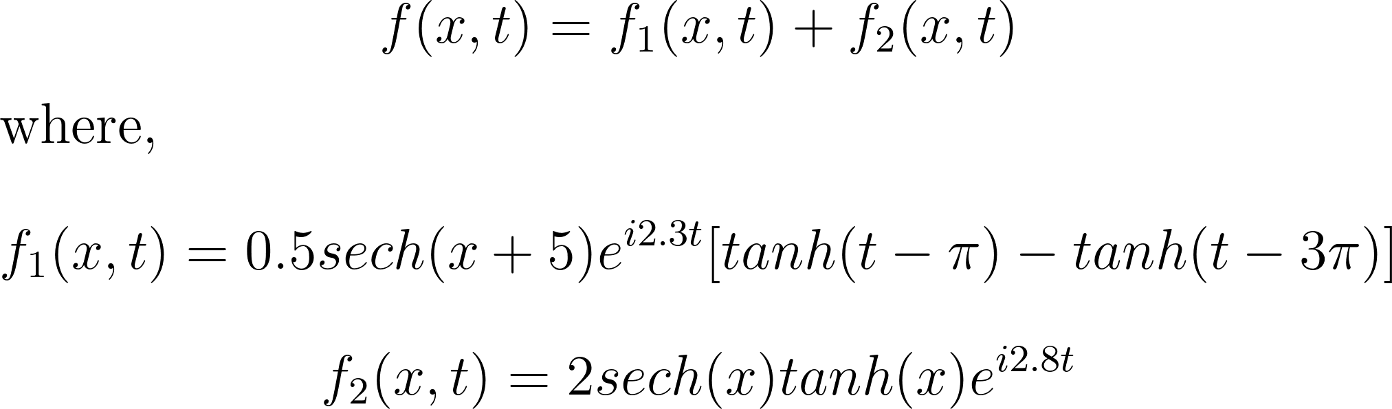
These signals have frequencies of ω1 = 2.3 and ω2 = 2.8, with the given corresponding spatial structures. Notice the signal f2, which turns on and off over time.

As before, you can generate the toy signal and visualize them using matplotlib.

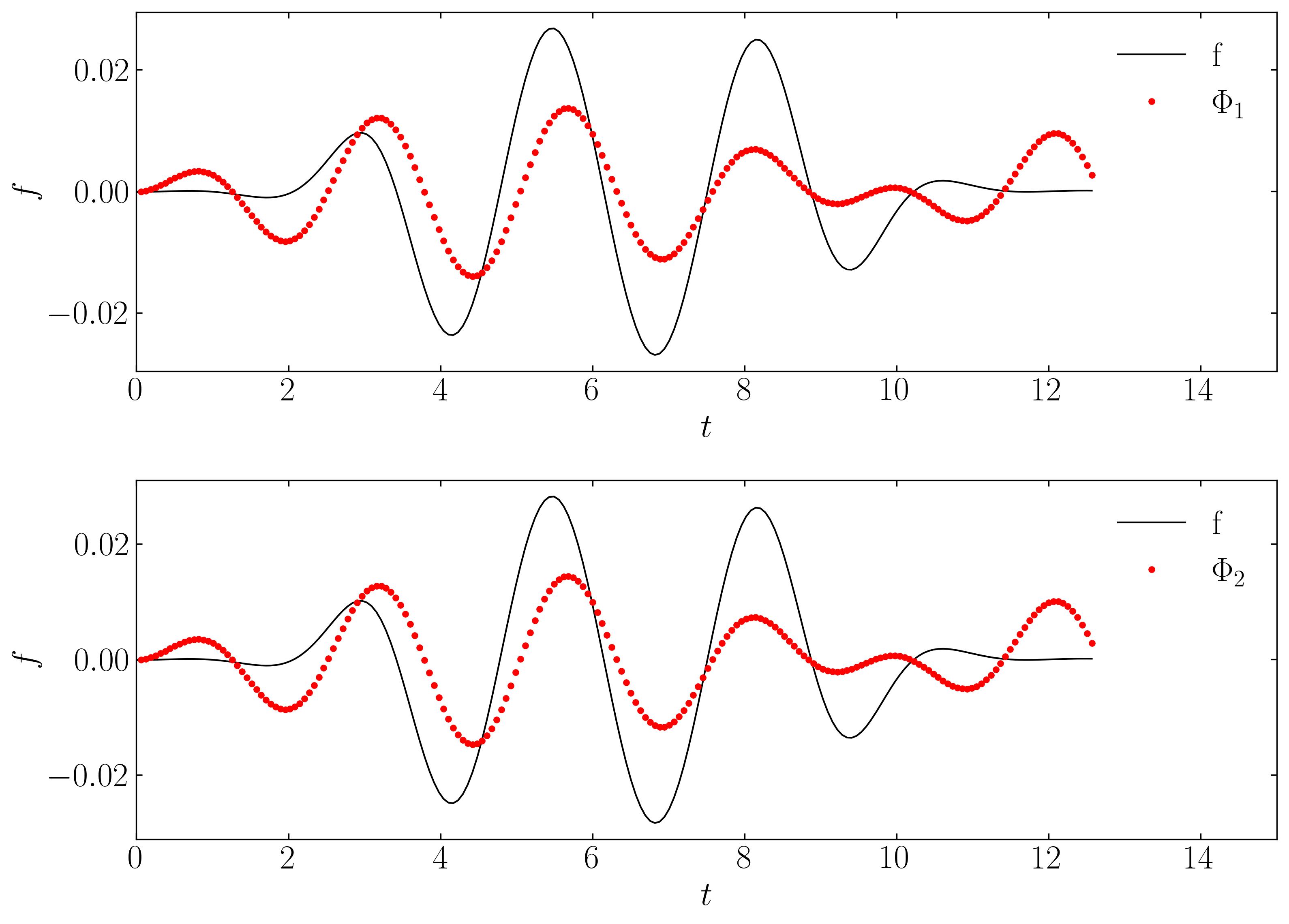
Next, compute the DMD and reconstruct the signal using a rank-10 approximation. The comparison between the original on-off mixed signal and the rank-10 DMD reconstruction is shown below:

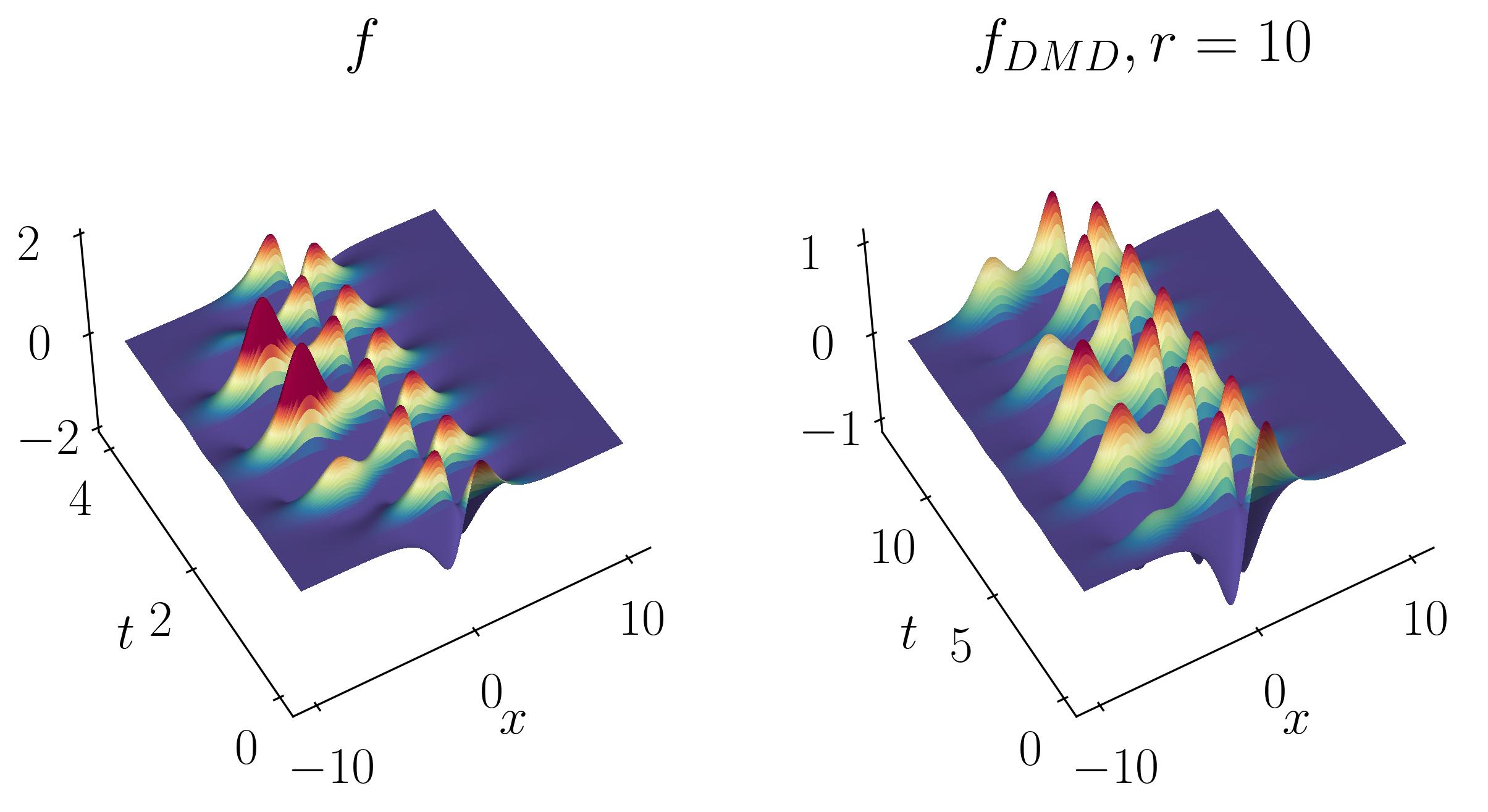
Interestingly, even at rank-10, DMD fails to capture the correct turn-on and turn-off behavior of the original signal. Specifically, DMD cannot approximate the spatial behavior of the on-off signal in Modes 1 and 2, as shown below:

Unlike translational or rotational invariance, which merely creates an artificially high dimension in DMD, this case shows DMD completely failing to characterize the correct dynamics. This limitation can also be addressed using mrDMD.

In conclusion, while Dynamic Mode Decomposition (DMD) is a powerful tool for analyzing complex dynamical systems, it has its limitations, particularly in handling translational invariances and transient phenomena. As demonstrated with our toy examples, traditional DMD can struggle with accurately capturing dynamics in cases involving movement or sudden changes. These limitations highlight the importance of extending DMD methodologies to more sophisticated versions like multiresolution DMD (mrDMD), which can better handle these challenges.