Proper Orthogonal Decomposition (POD) has long been a cornerstone in data-driven analysis, offering valuable insights into the dominant structures of complex systems. However, POD often falls short when dealing with systems exhibiting rich temporal dynamics. This is where Spectral Proper Orthogonal Decomposition (SPOD) shines. By incorporating frequency information into the analysis, SPOD unveils a deeper understanding of the underlying mechanisms driving system behavior. In this blog, we’ll explore how SPOD transcends the limitations of POD, unlocking new avenues for exploration and discovery.

Large, complex and non-linear datasets often contain intricate patterns that evolve over time and space, patterns which cannot be easily recognized. These patterns are crucial for understanding complex systems in nature, such as atmospheric evolution, turbulent flows, and plate tectonics. Identifying these coherent structures is essential for developing models that can predict scenarios which would otherwise remain elusive. In this context, dynamical systems theory, enhanced by recent advances in machine learning and data mining, is making significant strides in extracting actionable insights from complex data. Techniques based on singular-value decomposition (SVD) are particularly promising, as they relate to reduced-order modeling and dynamical systems.

In my previous articles, I have extensively discussed two versatile extensions of SVD: Proper Orthogonal Decomposition (POD) and Dynamic Mode Decomposition (DMD). However, POD has certain limitations. For instance, while POD can easily identify large coherent structures in a large dataset, it struggles to detect small repeating patterns, such as minor flow structures in turbulence, due to their low energy making them difficult to identify in the POD spectrum. This is where variants like Spectral Proper Orthogonal Decomposition (SPOD) come into play.

Spectral Proper Orthogonal Decomposition (SPOD) addresses this limitation by offering a frequency-resolved perspective. By decomposing data into frequency-specific modes, SPOD provides a more comprehensive understanding of system behavior, enabling researchers to identify dominant frequencies, mode shapes, and energy distributions. This enhanced insight enables a deeper insight into the underlying physics and mechanisms driving complex phenomena.

The fundamental idea of SPOD dates back to the 1960s, a recently developed algorithm by Towne et al. 2018 has revitalized its application. It is now used to study pedestrian-level wind environments, pollutant dispersion, and indoor ventilation in architectural and built environments.

In this and the next few articles, we will dive into the complex mathematics and applications of SPOD. Since I come from the background of fluid dynamics, my discussions on this topic include a lot of references to fluid flow, turbulence and flow dynamics in general.

Let’s begin!

Idea

In SPOD, the procedures of POD are carried out in the frequency domain, identifying the most energetic mode at discrete frequencies. This allows small structures to be found at their characteristic frequencies. SPOD differs from other SVD-based techniques in that it is derived from a standard (space-time) POD problem for stationary data. This leads to modes that are time-harmonic, oscillate at a single frequency, are coherent in both time and space, optimally represent the space-time statistical variability of the underlying stationary random processes, and are orthogonal both spatially and in space-time. Moreover, SPOD relates to DMD in that SPOD modes are optimally averaged DMD modes obtained from an ensemble DMD problem for stationary flows. Consequently, SPOD modes represent dynamic structures similar to DMD modes but also optimally account for the statistical variability of turbulent flows.

Mathematical Infrastructure

SPOD combines elements of Proper Orthogonal Decomposition (POD) and Fourier analysis to decompose a time series of spatial data into dominant frequency-dependent modes. These modes can be used for data compression, noise reduction, and identifying coherent structures within the data. Mathematically, SPOD modes are eigenvectors of the cross-spectral density (CSD) matrix at each frequency, with the eigenvalues corresponding to the energy of each mode at a distinct frequency.

Schematically, SPOD appears straightforward as shown below. However, the mathematical and fundamental aspects of SPOD can become quite complex quickly.

As is always the case with data-driven dynamical system analysis, we begin with data collection and preprocessing. Suppose we have a time series of data, denoted as $q(x,t)$, where $x$ represents the spatial coordinates and $t$ denotes time. To simplify, let’s assume this time series consists of velocity field (u and v) measurements gathered across different spatial points ($x_1, x_2, …, x_n$) and time intervals ($t_1, t_2, …, t_m$):

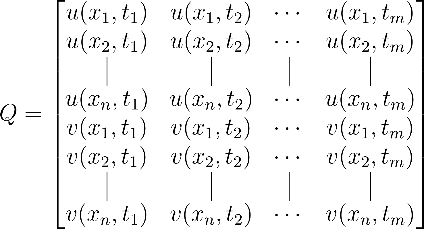
For simplicity, let’s assume that the data matrix looks as follows:

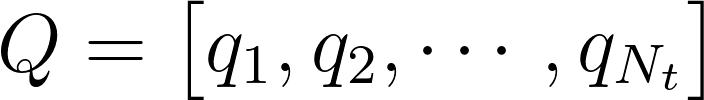
where $N_t$ is the total number of snapshots and $q_i$ denotes a time-instant of flow field (Snapshot).

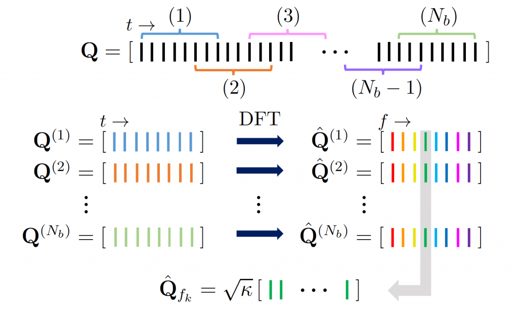
This data matrix $Q$ is then divided into $N_b$ overlapping or non-overlapping segments, such that $N_b \ll N_t$, by applying the Welch periodogram method, with each block consisting of $N_f$ snapshots. Each block is assumed to be a statistically independent realization under the ergodicity hypothesis.

he discrete Fourier transform (DFT) is performed on each block to convert the problem to the frequency domain. To avoid spectral leakage, each block is windowed using the Hamming window function and overlapped with neighboring blocks. The resultant matrix for the $j^{th}$ block will looks as follows:

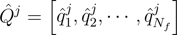
At this stage, $N_f$ is equivalent to the number of resolved frequencies since we have now converted the problem into the frequency domain!!

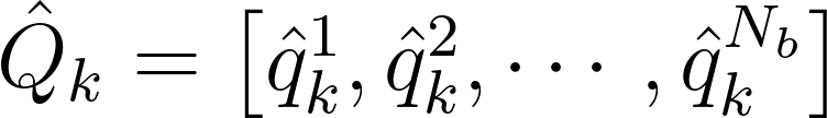
Next, the frequency-domain matrices of blocks are reshaped according to the frequency. For the $k^{th}$ frequency, the corresponding matrix is

Then one can simply compute the cross-spectral density (CSD) matrix for each frequency as follows:

where W is the weight matrix for scaling of different flow variables, and determines the physical meaning of the SPOD mode energy.

Finally, eigenvalue decomposition is performed on the weighted CSD matrix for each frequency as follows:

Here, The eigenfunctions $\phi_k$ corresponding to the largest eigenvalues $\lambda(f)$ represent the dominant spatial structures at frequency $f$. These are the SPOD modes.

In summary, SPOD combines Fourier analysis and POD to decompose a time series of spatial data into dominant frequency-dependent modes, which can be used for data compression, noise reduction, and identifying coherent structures in the data. In my next article, I will showcase a toy code for SPOD to better understand these steps.