Implementing Spectral Proper Orthogonal Decomposition in Python

Understanding the theory behind Spectral Proper Orthogonal Decomposition (SPOD) is essential, but practical implementation often poses challenges. This blog provides a hands-on approach by sharing a step-by-step code example. By following this guide, readers can apply SPOD to their own datasets, gaining valuable insights into complex systems.

Spectral Proper Orthogonal Decomposition (SPOD) stands at the intersection of spectral analysis and dimensionality reduction, offering a powerful tool for uncovering dominant structures in complex datasets. While the theoretical foundation of SPOD is crucial for understanding its potential, the practicalities of implementation can often be daunting. This blog bridges that gap, providing a clear, hands-on approach to SPOD through a detailed, step-by-step code example. Whether you’re working with fluid dynamics, signal processing, or any field involving large-scale data, this guide will equip you with the practical skills to apply SPOD to your own datasets, unveiling the intricate patterns and insights hidden within.

Test Case

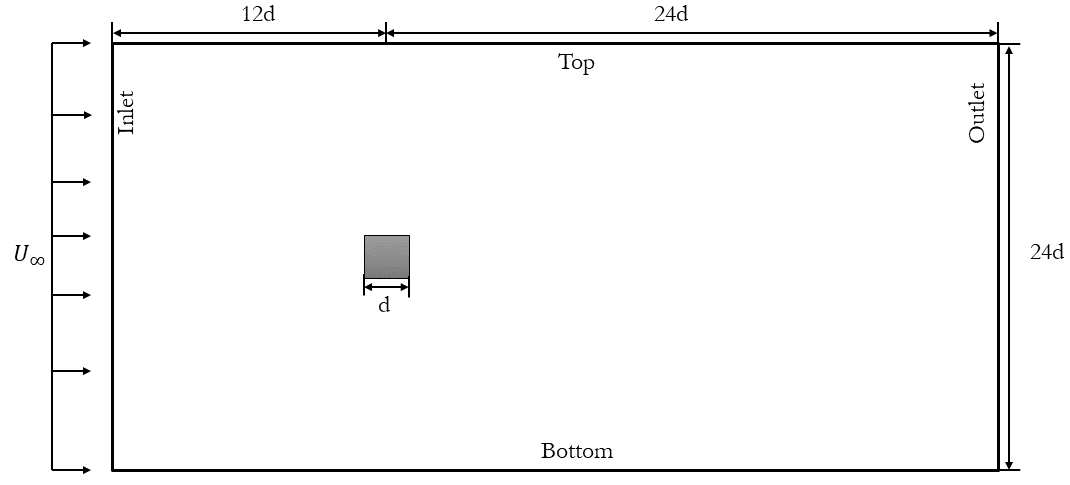
The test case I will explore for Spectral Proper Orthogonal Decomposition (SPOD) involves the dynamics of a two-dimensional flow around a square cylinder at a Reynolds number of 100. This flow will be simulated using Direct Numerical Simulations (DNS) implemented in OpenFOAM. The setup of this case will closely adhere to the configuration outlined by Bai and Alam (2018) for reference. A visual representation of the domain is provided below:

The choice of this specific case is deliberate. The wake generated behind the cylinder is a classic example of periodic (Kármán) vortex shedding. This phenomenon manifests as a repetitive shedding of vortices, resulting in a periodic flow regime characterized by a dominant frequency and its harmonics. These inherent characteristics make it an ideal candidate for modal decomposition investigations. Additionally, by replicating a published case, we can effectively scrutinize and validate the underlying flow physics within our simulations.

A comprehensive guide to preparing your OpenFOAM case for Modal Decompositions is available here, offering detailed insights into the necessary steps.

Extracting data from simulation

The first step is to extract data from your simulation. To do this, simply follow my previous post.

Or, follow along by opening up a Jupyter notebook and importing the necessary modules, including PyVista:

import matplotlib.colors
import matplotlib.pyplot as plt
import numpy as np
import pandas as pd
import fluidfoam as fl
import scipy as sp
import os
import pyvista as pv
import imageio
import io

%matplotlib inline
plt.rcParams.update({'font.size' : 18, 'font.family' : 'Times New Roman', "text.usetex": True})

Setting Path Variables and Constants:

### Constants
d = 0.1
Ub = 0.015

### Paths
Path = 'E:/Blog_Posts/Simulations/Sq_Cyl_Surfaces/surfaces/'
save_path = 'E:/Blog_Posts/SquareCylinderData/'

Files = os.listdir(Path)

Now, let’s attempt to read the first snapshot surface using PyVista:

Data = pv.read(Path + Files[0] + '/zNormal.vtp')
grid = Data.points
x = grid[:,0]
y = grid[:,1]
z = grid[:,2]
rows, columns = np.shape(grid)
print('rows = ', rows, 'columns = ', columns)

print(Data.array_names)

Output:

['TimeValue', 'p', 'U']

Here, we observe that our 2D slices encompass velocity and pressure fields. Leveraging PyVista, we can extract the vorticity field for each snapshot and organize the resulting data into a large, tall, and slender matrix to facilitate POD computation.

Data = pv.read(Path + Files[0] + '/zNormal.vtp')
grid = Data.points
x = grid[:,0]
y = grid[:,1]
z = grid[:,2]
rows, columns = np.shape(grid)
print('rows = ', rows, 'columns = ', columns)

### For U
Snaps = len(Files) # Number of snapshots
data_Vort = np.zeros((rows,Snaps-1))
for i in np.arange(0,Snaps-1):
    data = pv.read(Path + Files[i] + '/zNormal.vtp')
    gradData = data.compute_derivative('U', vorticity=True)
    grad_pyvis = gradData.point_data['vorticity']
    data_Vort[:,i:i+1] = np.reshape(grad_pyvis[:,2], (rows,1), order='F')

np.save(save_path + 'VortZ.npy', data_Vort)

Let’s examine the size of the matrix we’re dealing with by querying the shape of the data_Vort array:

data_Vort.shape
### OUTPUT
### (96624, 1600)

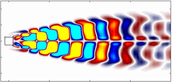
Additionally, we can visualize a snapshot of the vorticity field:

Moreover, for a more dynamic representation (showing off, in other words), we can animate the vorticity field:

POD and most dominant modes

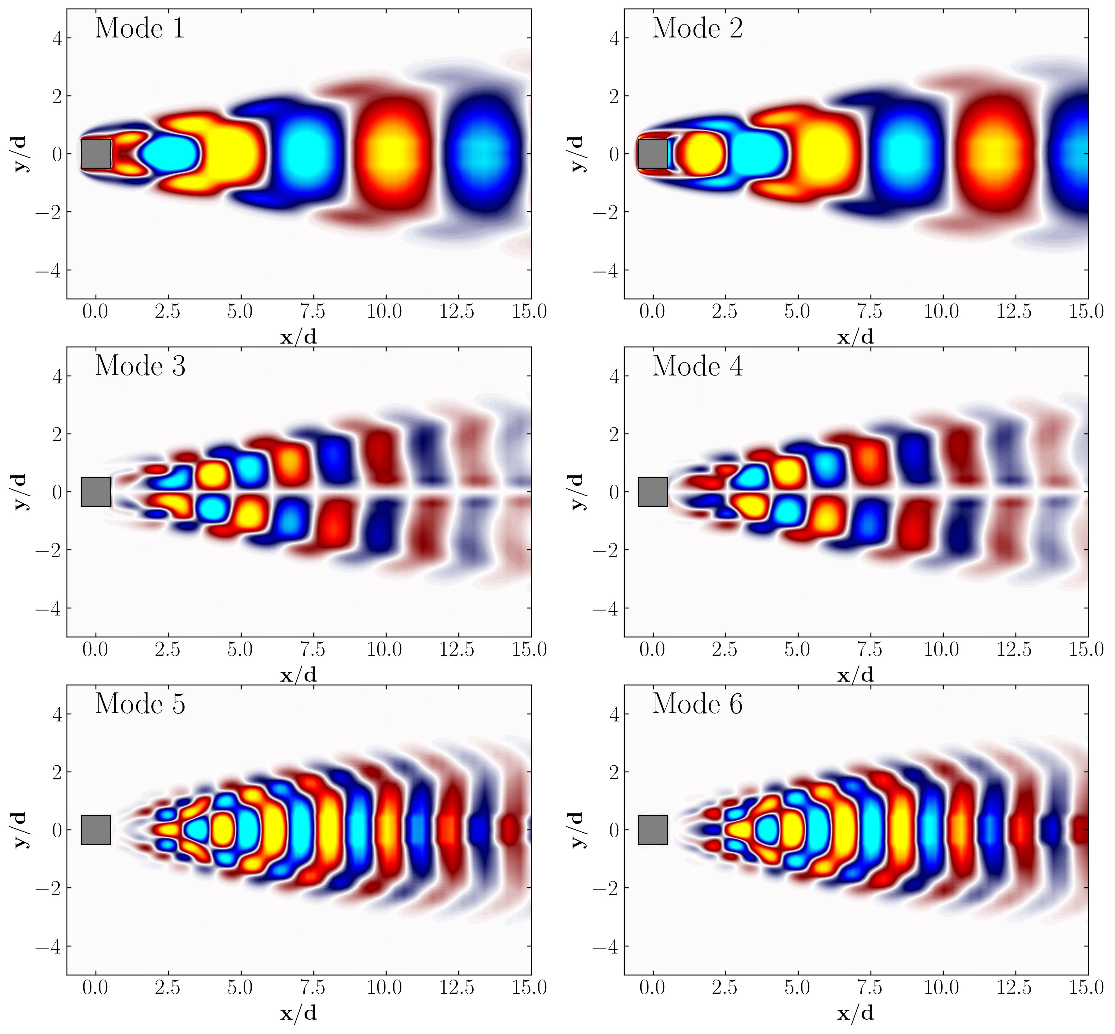
When considering the simple Proper Orthogonal Decomposition (POD) of the flow around a square cylinder at a Reynolds number of 100, the most dominant POD modes are as follows:

Furthermore, these modes are associated with characteristic frequencies as illustrated below:

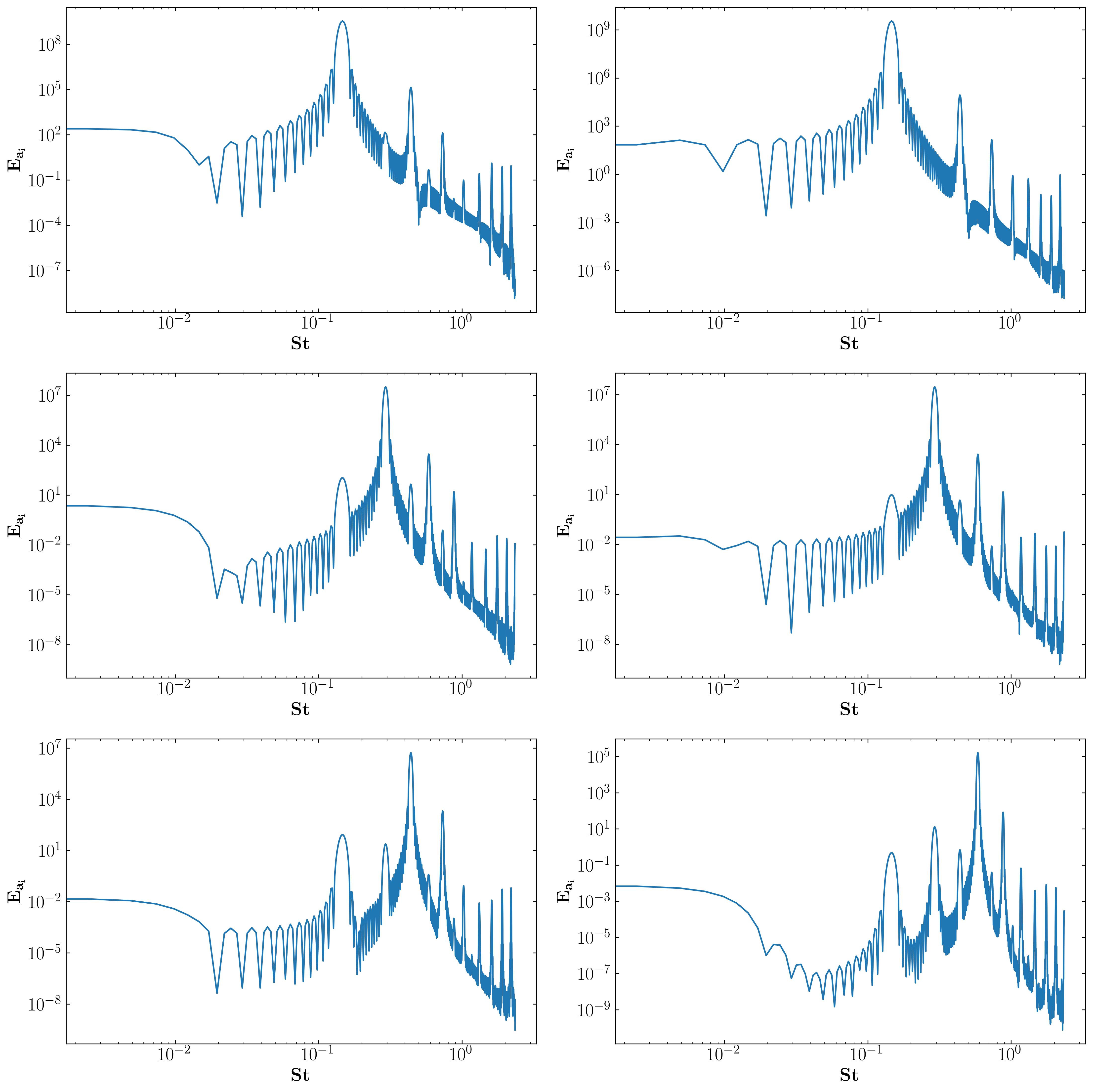
These characteristic frequencies manifest in the overall flow, as demonstrated by the FFT of a velocity probe near the square cylinder:

These results will aid us in developing a small toy code for SPOD.

SPOD Toy Code

To generate the toy code, let’s first obtain a mean-removed data matrix as follows:

MeanVort = np.mean(data_Vort, axis=1)
VortPrime = data_Vort - MeanVort[:,np.newaxis]
VortPrime.shape

Dividing the data into overlapping segments is a critical step in Spectral Proper Orthogonal Decomposition (SPOD) for several reasons, each contributing to the robustness and accuracy of the analysis.

1. Overlapping Segments

• Increased Statistical Reliability: By using overlapping segments, you effectively increase the number of data points without requiring additional data collection. This provides more samples for computing the cross-spectral density (CSD) matrix, leading to better statistical reliability and reducing variance in the estimates.
• Improved Frequency Resolution: Overlapping segments allow for a finer resolution in the frequency domain. When Fourier transforms are applied to these segments, overlapping ensures that subtle frequency components are captured more accurately, enhancing the spectral analysis.
• Smoothing Effects: Overlapping introduces a smoothing effect in the spectral estimates, which can help in mitigating the effects of noise and transient components in the data. This makes the resulting SPOD modes more robust and representative of the underlying physical phenomena.

1. Non-Overlapping Segments

• Computational Efficiency: Non-overlapping segments are computationally less intensive compared to overlapping ones because each data point is used only once. This can be beneficial when dealing with very large datasets or limited computational resources.
• Simplicity and Independence: Using non-overlapping segments simplifies the implementation and ensures that each segment is independent. This can be particularly useful when the temporal independence of segments is critical for the analysis.
• Distinct Time Windows: Non-overlapping segments provide distinct time windows, which can be advantageous when the objective is to study the evolution of patterns over non-overlapping time intervals. This helps in understanding how the dominant structures change over different periods.

There is a trade-off between the increased statistical reliability and computational cost when choosing between overlapping and non-overlapping segments. The choice depends on the specific requirements of the analysis, the size of the dataset, and the available computational resources. Moreover, length of each segment (whether overlapping or non-overlapping) should be chosen based on the dominant frequencies of interest. Longer segments provide better frequency resolution but at the cost of temporal resolution, while shorter segments offer better temporal resolution but poorer frequency resolution.

Let’s consider overlapping segments in this case, specifically with a 99% overlap.

nBlocks = 256
nTotal = VortPrime.shape[1]

Next, we’ll input the time-step of sampling, extract the related frequencies, and convert these frequencies into the Strouhal Number as follows:

dt = 0.01*142
f = np.fft.fftfreq(nTotal, dt)
St = f*d/Ub

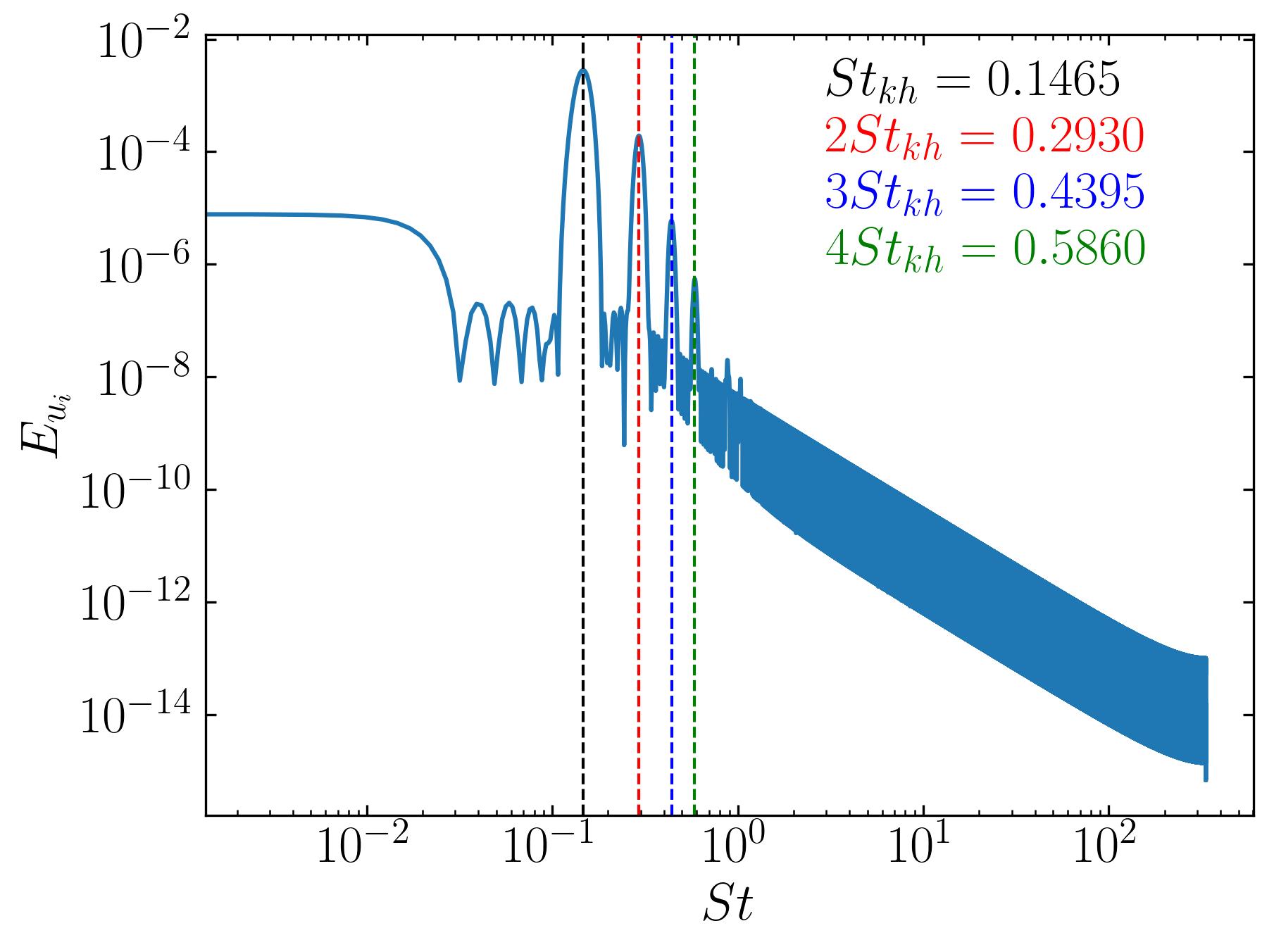
The list of Strouhal Numbers includes the dominant frequency and its harmonics, as shown in the FFT spectrum below:

The simple concept behing SPOD is that it combines elements of Proper Orthogonal Decomposition (POD) and Fourier analysis. Lets consider the SPOD algorithm for a single frequency, for example the second-harmonic in the figure above. Spectral Proper Orthogonal Decomposition (SPOD) at a single frequency identifies the dominant spatial structures that oscillate at that specific frequency within a dataset. By computing the cross-spectral density matrix for this frequency and solving the associated eigenvalue problem, SPOD extracts the primary modes, revealing coherent patterns and reducing noise. This technique highlights key dynamics tied to the chosen frequency, offering focused insights into complex systems.

To generate this toy SPOD code for a single frequency, we will divide the data into segments, convert the data into the frequency domain, and then collect them at a specific frequency, such as the second harmonic.

for i in range(0, nBlocks):
    Q1n = VortPrime[:, 0:nTotal-nBlocks + i]
    Q1n_star = np.fft.fft(Q1n, axis = 1)
    Q1New[:,i] = Q1n_star[:,120]

This new matrix, Q1New, is our data matrix in the frequency domain. We will use this matrix to compute the Cross-Spectral Density (CSD) Matrix, which is essentially a correlation matrix in POD.

M = np.dot(Q1New.conj().T, Q1New)/nBlocks

Finally, we can solve the eigenvalue problem for the CSD matrix to obtain the SPOD modes for the second harmonic:

[Lambda, Theta] = np.linalg.eig(M)
Modes = np.dot(np.dot(Q1New, Theta), np.diag(1/np.sqrt(Lambda)/np.sqrt(nBlocks)))

Then, one can easily plot the SPOD modes for the second harmonic using simple plotting routines in Matplotlib as follows:

Rect1 = plt.Rectangle((-0.5, -0.5), 1, 1, ec='k', color='white', zorder=2)

fig, ax = plt.subplots(figsize=(11, 4))
p = ax.tricontourf(x/0.1, y/0.1, np.real(Modes[:,0])*(d/Ub), levels = 1001, 
                   vmin=-0.02, vmax=0.02, cmap = cmap)
ax.add_patch(Rect1)
ax.xaxis.set_tick_params(direction='in', which='both')
ax.yaxis.set_tick_params(direction='in', which='both')
ax.xaxis.set_ticks_position('both')
ax.yaxis.set_ticks_position('both')
ax.set_xlim(-1, 20)
ax.set_ylim(-5, 5)
ax.set_aspect('equal')
ax.set_xlabel(r'$\bf x/d$')
ax.set_ylabel(r'$\bf y/d$')
plt.show()

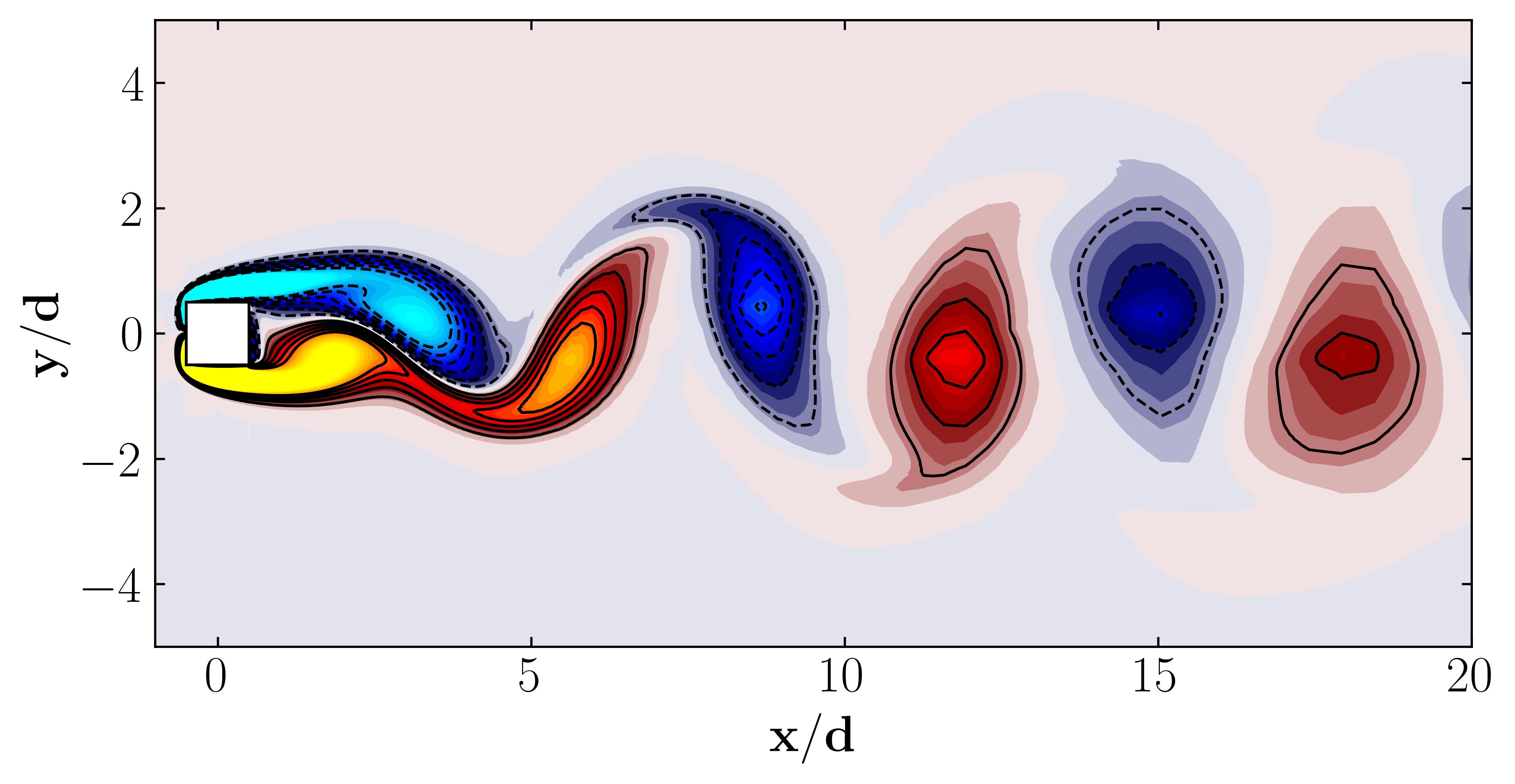
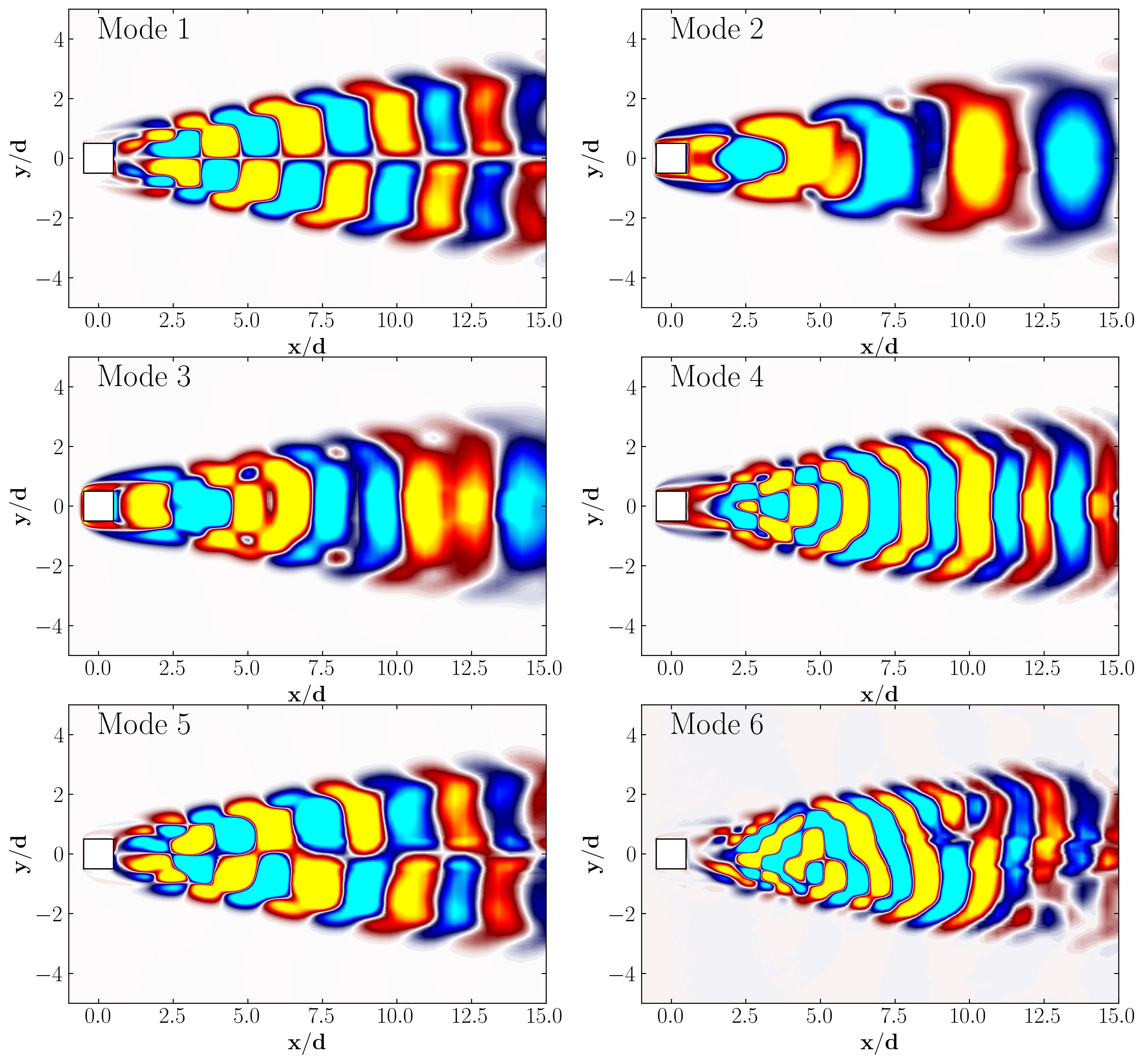
Here are the first 6 SPOD modes for the second harmonic, highlighting the dominant spatial structures that oscillate at that specific frequency within the complex flow around a square cylinder:

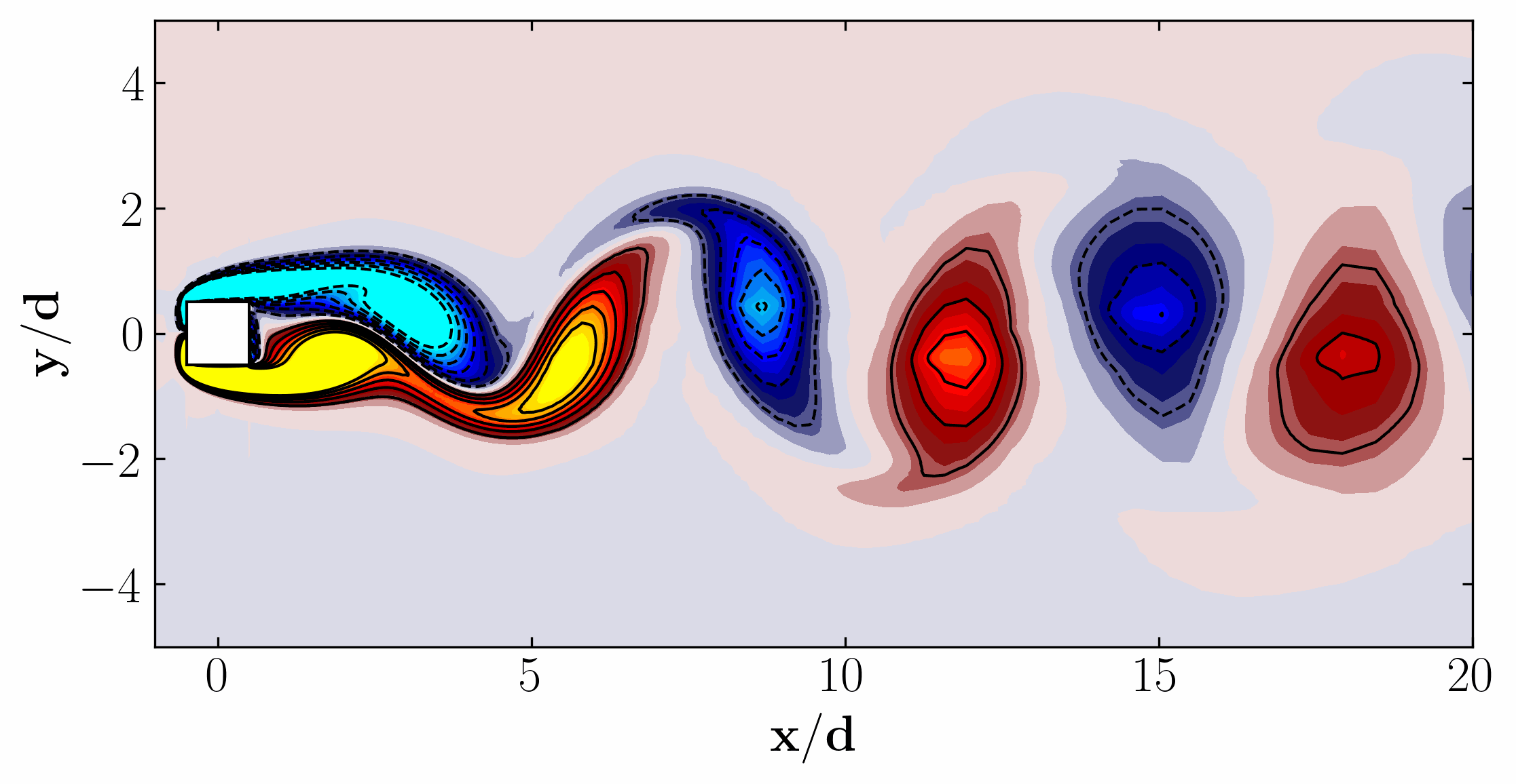
Similarly, here are the first 6 SPOD modes corresponding to the dominant vortex shedding frequency:

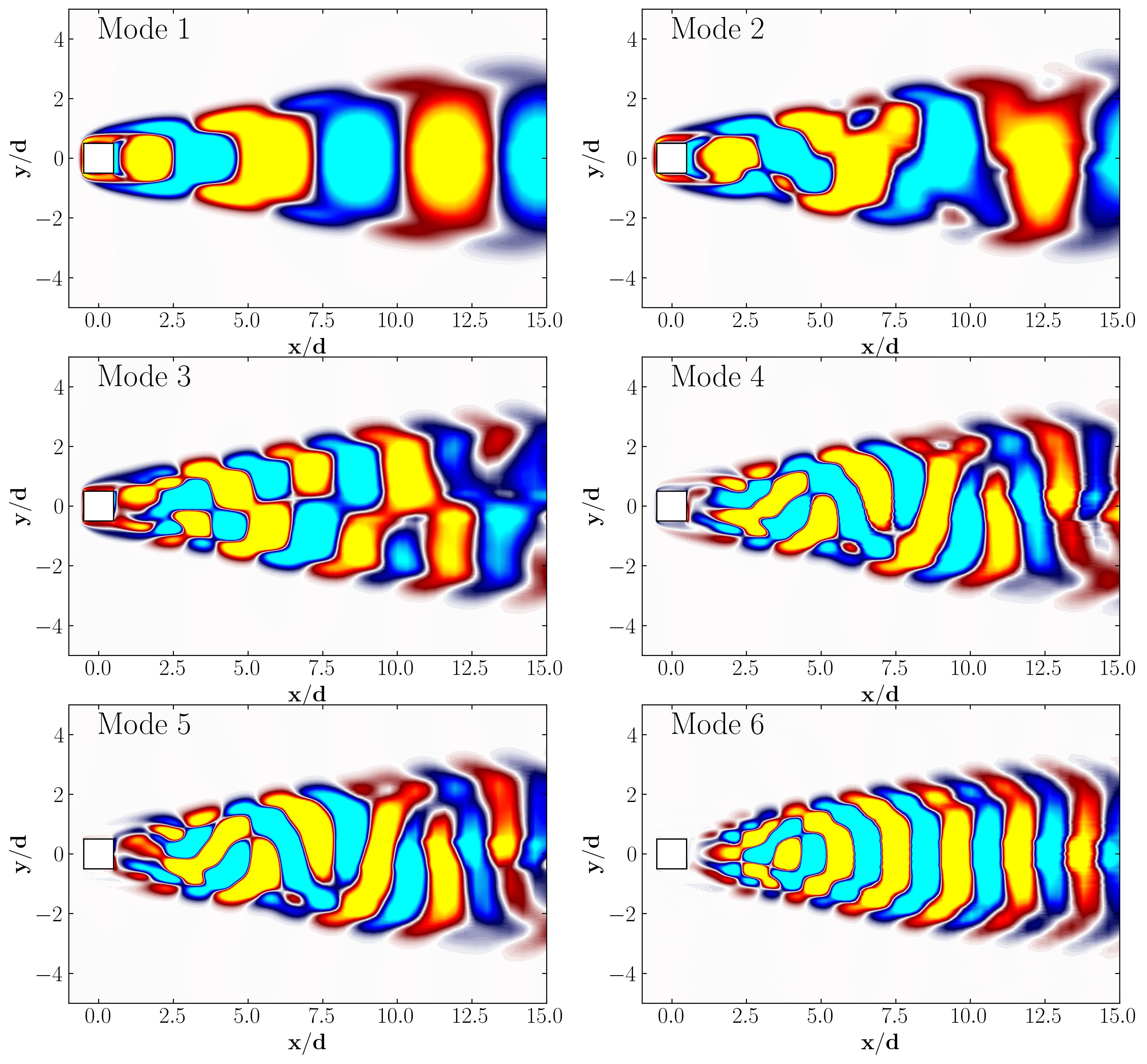
Notice that Mode 1 for both the dominant and second harmonic frequencies closely correlates with POD Modes 1 and 3, which are associated with these specific frequencies.

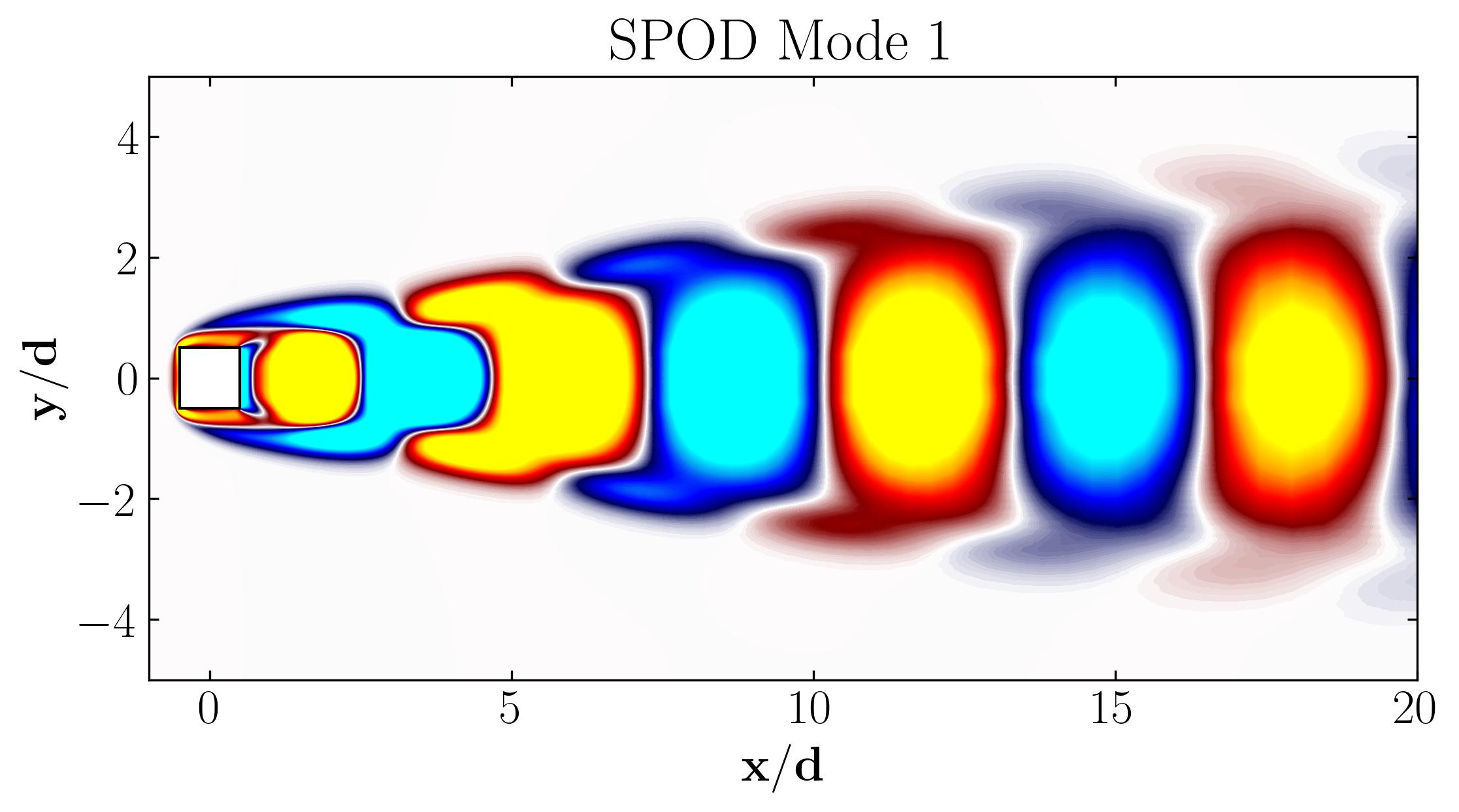
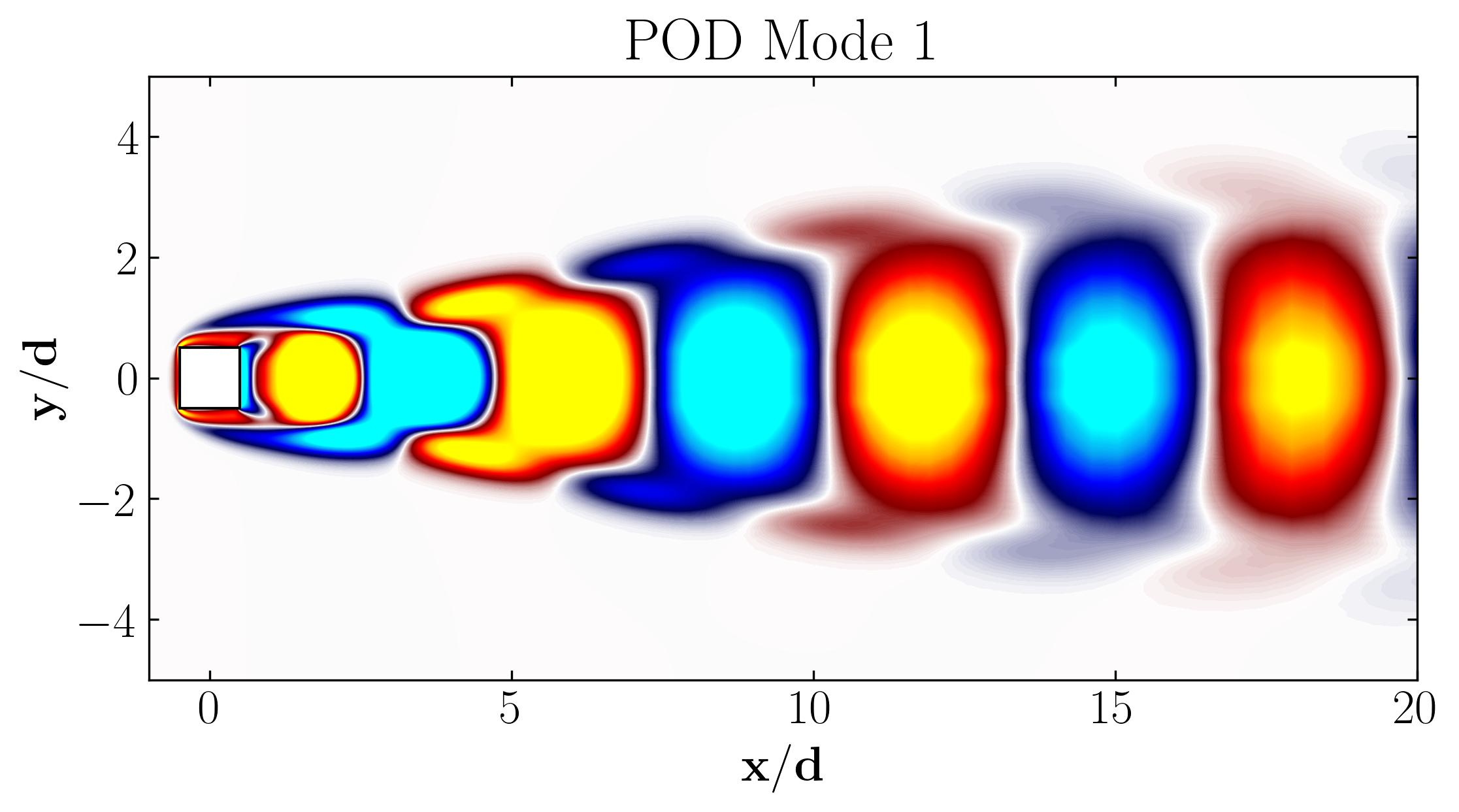
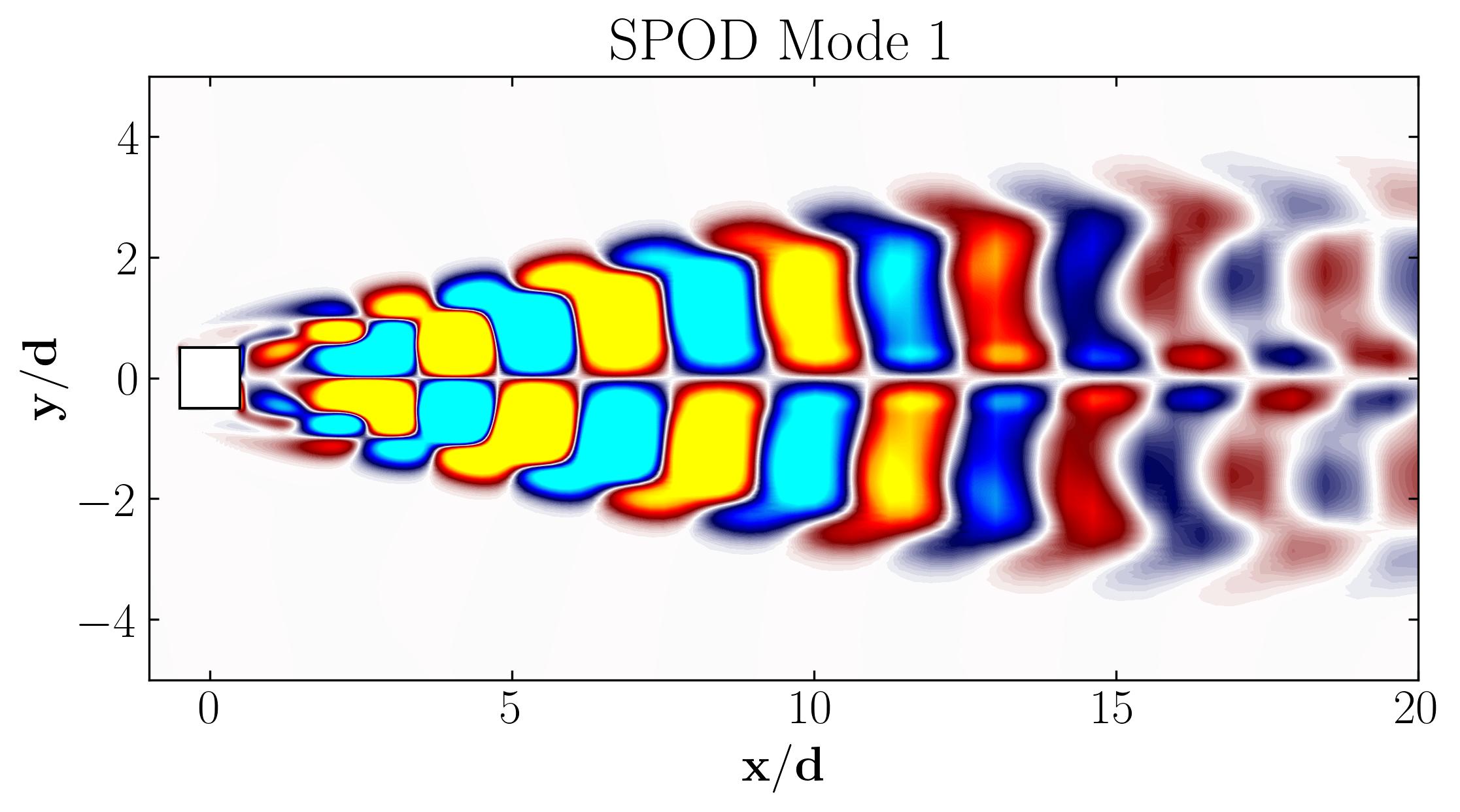
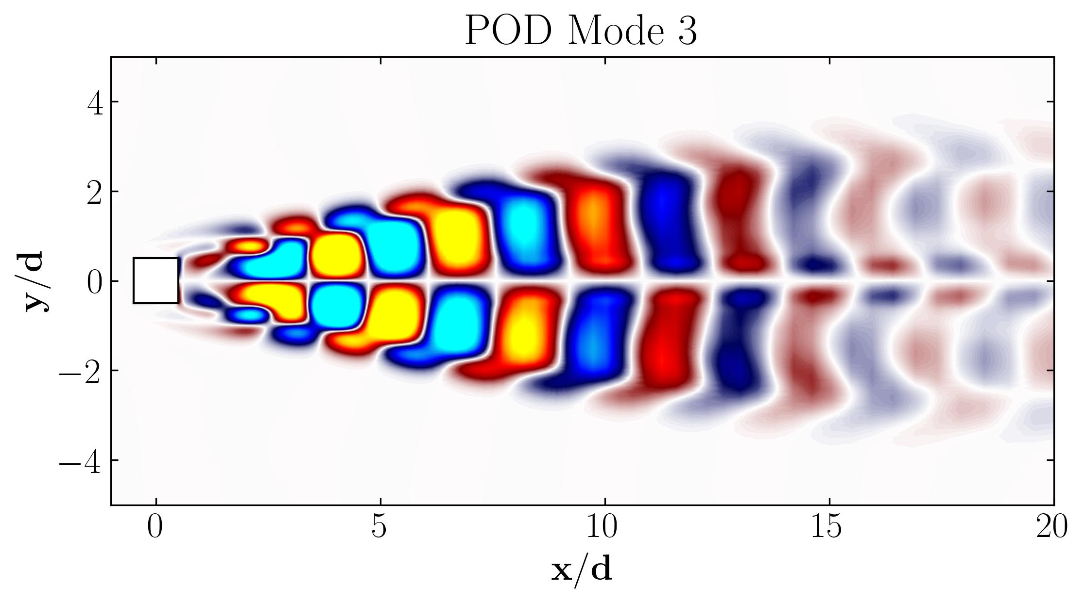
This suggests that the spatial structures identified by SPOD at these specific frequencies are similar to those captured by POD. This close correlation suggests that the energy-dominant structures in the dataset (captured by POD) are primarily driven by the dynamics at the dominant frequency and its second harmonic, for example. It also highlights the effectiveness of SPOD in isolating these structures at specific frequencies, which may be more challenging to discern with POD alone. Further, the connection between SPOD and POD modes can help in understanding the multi-scale nature of the flow or system being analyzed, where certain modes are prominent across different scales and frequencies.

In my next article, I will focus on the complete SPOD algorithm, which considers all frequencies and their associated spatial structures, and explore its application in fluid flow problems.