Capturing a spatio-temporal phenomenon using Spectral Proper Orthogonal Decomposition (SPOD) and OpenFOAM
Spectral Proper Orthogonal Decomposition (SPOD) is a powerful technique for uncovering the dominant spatial patterns within a dataset at specific frequencies. By analyzing a single frequency, we can identify the key structures responsible for the oscillations at that point in the spectrum. However, to gain a comprehensive understanding of the multi-scale nature of a flow, we must consider the entire frequency range. In this article, lets explore the complete SPOD algorithm, which explores all frequencies and their associated spatial modes, using OpenFOAM simulation data.
Understanding complex fluid flows is a cornerstone of many scientific and engineering disciplines. To unravel the intricate patterns and structures within these flows, researchers often turn to advanced data analysis techniques. One such method, Spectral Proper Orthogonal Decomposition (SPOD), has emerged as a valuable tool for extracting coherent structures across a range of frequencies. By applying SPOD to a dataset, we can decompose the flow into its constituent spatial modes and their corresponding spectral content, providing crucial insights into the underlying physics.
In this article, we will explore the complete SPOD algorithm, exploring its practical implementation in Python. By examining both single-frequency and full-spectrum analysis, we will demonstrate the power of SPOD in uncovering the multi-scale dynamics of complex flows.
Lets begin!!
The Code
Building on our previous exploration of SPOD programming in Python, this article takes advantage of a pre-existing implementation to streamline the process. We’ll leverage the well-developed SPOD Python code created by HexFluid named SPOD Python. This repository offers a comprehensive Python implementation of SPOD and includes various test cases based on published studies and datasets. By utilizing this established code, we can focus on the practical application of SPOD, saving time and ensuring accuracy.
Test Case
Continuing our exploration of SPOD, we will apply the code to a canonical flow problem: two-dimensional flow past a square cylinder at a Reynolds number of 100. This flow was simulated using Direct Numerical Simulations (DNS) within the OpenFOAM framework. For detailed guidance on preparing your OpenFOAM cases for modal decomposition, refer to this article.
Important Note: Overlapping Segments for Robust SPOD
Properly dividing a dataset into overlapping segments is crucial for accurate Spectral Proper Orthogonal Decomposition (SPOD). By computing the cross-spectral density (CSD) matrix using overlapping segments, we enhance statistical reliability, reduce variance in estimates, and achieve finer frequency resolution. A 50% overlap is commonly recommended to improve the robustness and representativeness of SPOD modes.
To obtain reliable SPOD results, a substantial amount of data spanning multiple vortex shedding cycles is essential. In this example, we utilized 50 vortex shedding cycles after reaching statistical convergence, gathering approximately 100 snapshots per cycle for a total of around 5000 snapshots.
Tip: For optimal efficiency, aim for a total number of snapshots that is a power of 2, for example $2^N$.
SPOD implementation
Assuming you’ve already collected and stored your data in a NumPy matrix named VortZ.npy as outlined in our previous article, let’s begin by launching a Jupyter Notebook and importing the required modules.
import matplotlib.colors
import matplotlib.pyplot as plt
import numpy as np
import pandas as pd
import fluidfoam as fl
import scipy as sp
import vmdpy as vmd
from numba import jit,njit
from matplotlib.colors import ListedColormap
import h5py
import os
import time
import spod
from matplotlib import cm
import io
import pyvista as pv

%matplotlib inline

plt.rcParams.update({'font.size' : 14, 'font.family' : 'Times New Roman', "text.usetex": True})
Don’t forget to clone the SPOD Python repository and include the spod module in your code.
Next, let’s configure the path variables and assign the .vtp slice files generated by OpenFOAM to a variable:
Path = 'E:/Blog_Posts/Simulations/Sq_Cyl_Surfaces/surfaces/'
save_path = 'E:/Blog_Posts/SPOD_SqCyl/'
dataPath = 'E:/Blog_Posts/SPOD_SqCyl/'
Files = os.listdir(Path)
Using the PyVista module, extract the data from a .vtp file to obtain the grid coordinates. Then, load the VortZ.npy matrix.
Data = pv.read(Path + Files[0] + '/zNormal.vtp')
grid = Data.points
x = grid[:,0]
y = grid[:,1]
z = grid[:,2]
data_Vort = np.load(dataPath + 'VortZ.npy')
rows, columns = np.shape(grid)
Snaps = np.shape(data_Vort)[1]
print('rows = ', rows, '\n', 'columns = ', columns, '\n', 'Snapshots = ', Snaps)
From the previous step, observe the output that shows the number of available snapshots
rows =  96624
columns =  3
Snapshots =  5360
This indicates that the dataset contains 96,624 degrees of freedom (spatial coordinates) and 5,360 snapshots (time instances). Such a large dataset is essential for robust SPOD analysis. In this example, I’ll be using the first 5,300 snapshots.
Let’s begin the SPOD implementation by first loading the data.
# Sec. 1 start time
start_sec1 = time.time()

grid = grid # grid points
ng = int(grid.shape[0])     # number of grid point
data = data_Vort[:, :5300].T
nt = data.shape[0]      # number of snap shot
nx = data.shape[1]      # number of grid point * number of variable
nvar = int(nx/ng)       # number of variables

# Sec. 1 end time
end_sec1 = time.time()

print('--------------------------------------'    )
print('SPOD input data summary:'                  )
print('--------------------------------------'    )
print('number of snapshot   :', nt                )
print('number of grid point :', ng                )
print('number of variable   :', nvar              )
print('--------------------------------------'    )
print('SPOD input data loaded!'                   )
print('Time lapsed: %.2f s'%(end_sec1-start_sec1) )
print('--------------------------------------'    )
Output:
--------------------------------------
SPOD input data summary:
--------------------------------------
number of snapshot   : 5300
number of grid point : 96624
number of variable   : 1
--------------------------------------
SPOD input data loaded!
Time lapsed: 0.00 s
--------------------------------------
Define the constants for the code:
d = 0.1 # Cylinder width
Ub = 0.015 # Flow Velocity
dt = 0.01*50 # Sampling time step for each snapshot
Finally, lets compute the SPOD using the spod module:
# Sec. 2 start time
start_sec2 = time.time()

# main function
spod.spod(data, dt, save_path, nDFT=512, method='fast')

# Sec. 2 end time
end_sec2 = time.time()

print('--------------------------------------'    )
print('SPOD main calculation finished!'           )
print('Time lapsed: %.2f s'%(end_sec2-start_sec2) )
print('--------------------------------------'    )
This step computes the block-wise DFT, lists all the frequencies in the spectrum, and stores the data in a file at the save_path location. Since this step involves the actual SPOD computation, it will be both time and memory intensive.
Next, read the SPOD results from the saved file and extract the modal energy (L), mode shapes (P), and frequency (f) into separate NumPy arrays for further analysis.
# -------------------------------------------------------------------------
# 3. Read SPOD result
# -------------------------------------------------------------------------

# Sec. 3 start time
start_sec3 = time.time()

# load data from h5 format
SPOD_LPf  = h5py.File(os.path.join(save_path,'SPOD_LPf.h5'),'r')
L = SPOD_LPf['L'][:,:]    # modal energy E(f, M)
P = SPOD_LPf['P'][:,:,:]  # mode shape
f = SPOD_LPf['f'][:]      # frequency
SPOD_LPf.close()

np.save(save_path + 'L_U50Modes_z0.npy', L)
np.save(save_path + 'f_U50Modes_z0.npy', f)
np.save(save_path + 'P_U50Modes_z0.npy', P)

# Sec. 3 end time
end_sec3 = time.time()

print('--------------------------------------'    )
print('SPOD results read in!'                     )
print('Time lapsed: %.2f s'%(end_sec3-start_sec3) )
print('--------------------------------------'    )
Next, lets plot the SPOD modal energy spectrum.
fig, ax = plt.subplots()

ax.loglog(f[0:-1]*d/Ub, L[0:-1,0])
ax.loglog(f[0:-1]*d/Ub, L[0:-1,1])
ax.loglog(f[0:-1]*d/Ub, L[0:-1,2])
ax.loglog(f[0:-1]*d/Ub, L[0:-1,3])
ax.loglog(f[0:-1]*d/Ub, L[0:-1,4])

xmax = f[np.argmax(L[0:-1,0])]
print("Strouhal Number = ", xmax*d/Ub)

ax.axvline(xmax*d/Ub, c='k', ls='--', lw=1)
ax.axvline(xmax*d/Ub*2, c='r', ls='--', lw=1)
ax.axvline(xmax*d/Ub*3, c='b', ls='--', lw=1)
ax.axvline(xmax*d/Ub*4, c='g', ls='--', lw=1)

ax.set_xlabel('Strouhal Number')
ax.set_ylabel('SPOD mode energy')

plt.show()
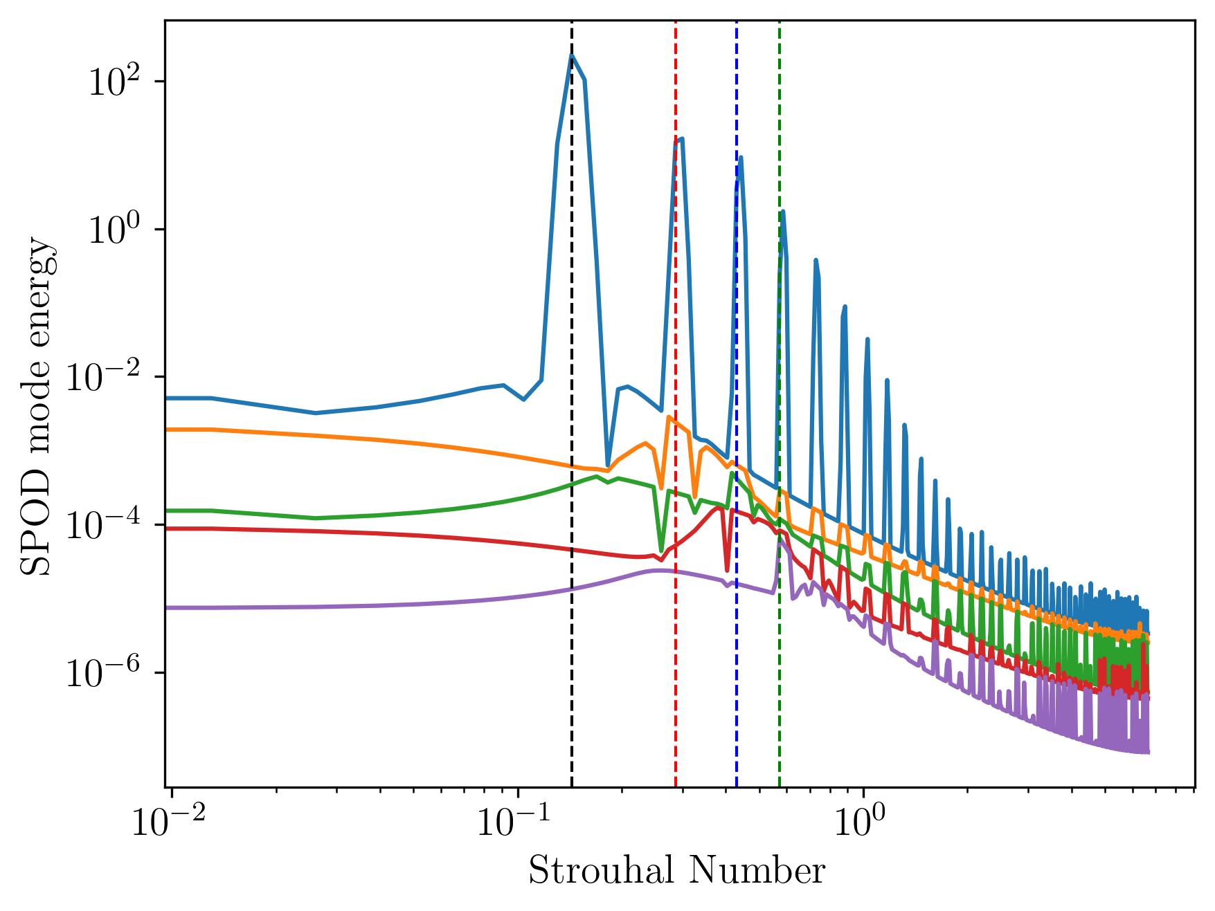
The spectrum reveals that the first five modes capture most of the energy, while the energy in the remaining modes is negligible. The bulk of the flow energy resides in large-scale, low-frequency components, with energy cascading down to smaller scales within the inertial subrange. Mode 1, in particular, dominates by containing a significant portion of the energy, highlighting a low-rank behavior that suggests a physically dominant mechanism is present in the flow field. This can be further understood by visualizing the modes.
To visualize the SPOD modes, start by selecting a frequency. You can do this by finding the index of the maximum frequency using np.where(f == xmax). Then, access the mode data using P[Freq, :, Mode], where Freq is the index of the selected frequency and Mode refers to the mode number.
Rect1 = plt.Rectangle((-0.5, -0.5), 1, 1, ec='k', color='white', zorder=2)

fig, ax = plt.subplots(figsize=(11, 4))

p = ax.tricontourf(x/0.1, y/0.1, np.real(P[11, :, 0])*d/Ub, levels = 1001,
                   vmin=-0.02, vmax=0.02, cmap = cmap.reversed())

ax.add_patch(Rect1)
ax.xaxis.set_tick_params(direction='in', which='both')
ax.yaxis.set_tick_params(direction='in', which='both')
ax.xaxis.set_ticks_position('both')
ax.yaxis.set_ticks_position('both')

ax.set_xlim(-1, 20)
ax.set_ylim(-5, 5)

ax.set_aspect('equal')
ax.set_xlabel(r'$\bf x/d$')
ax.set_ylabel(r'$\bf y/d$')

plt.show()
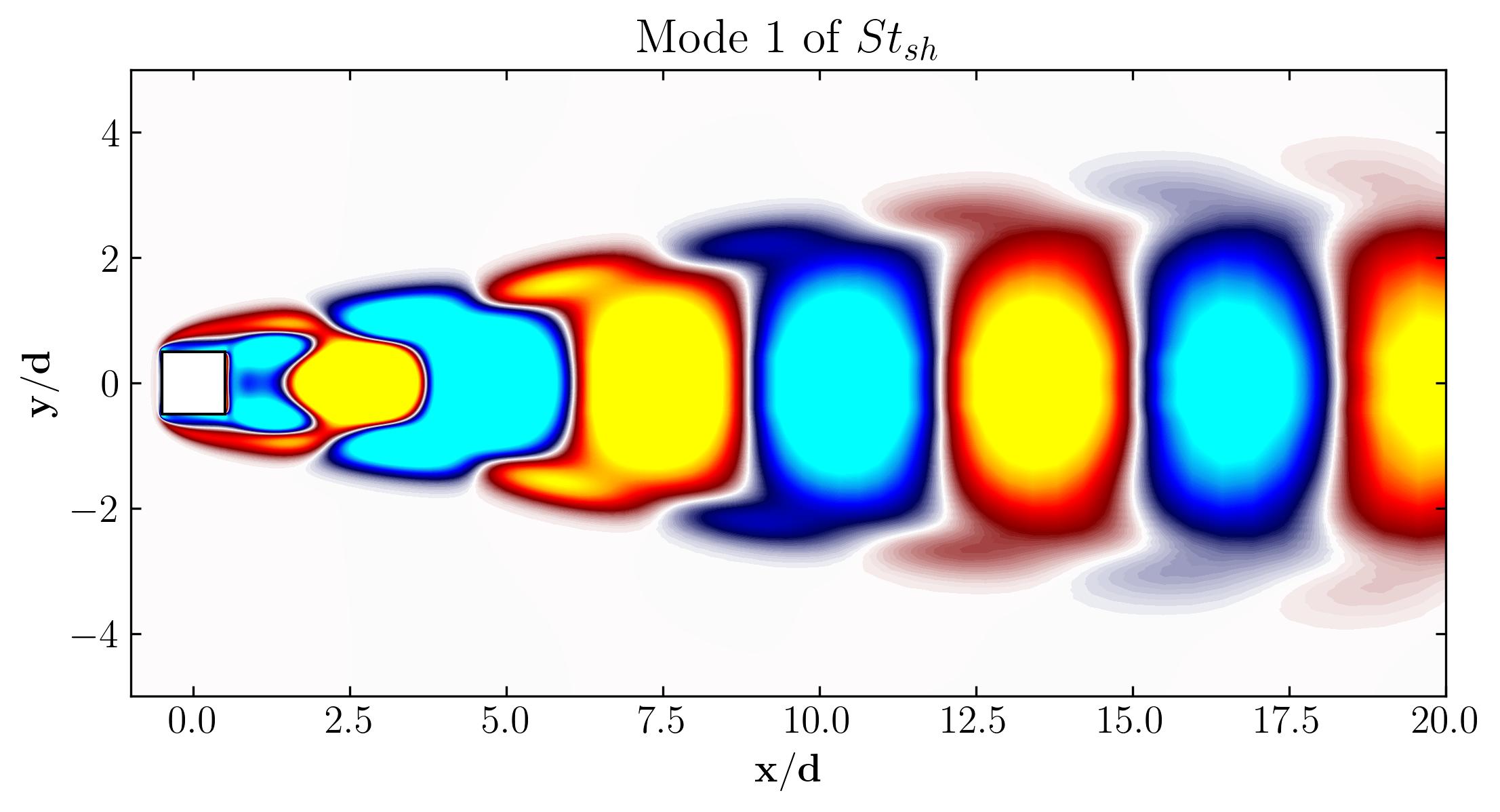
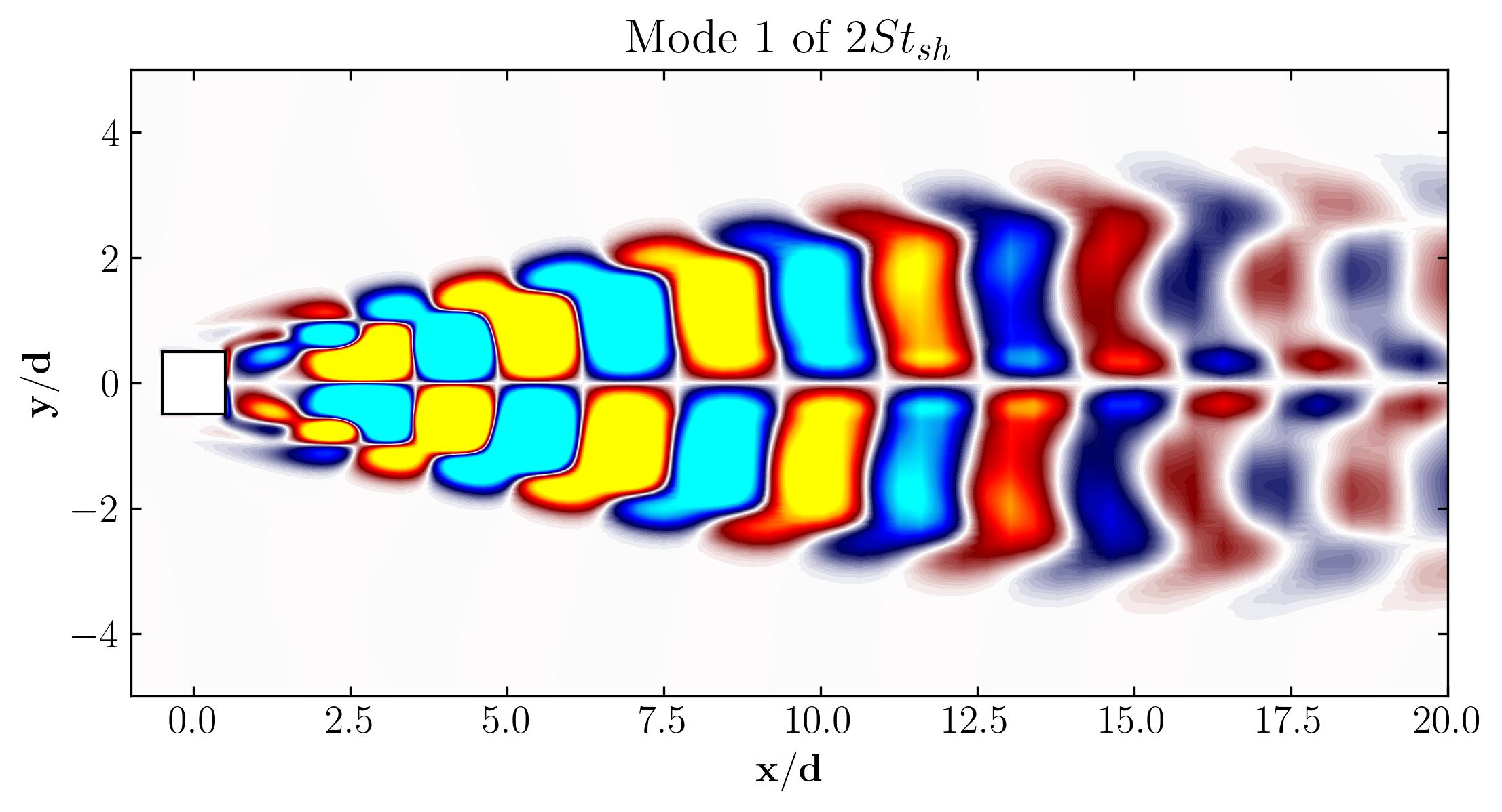
For example, Mode 1 for the dominant frequency and its second harmonic in the spectrum appear as follows:
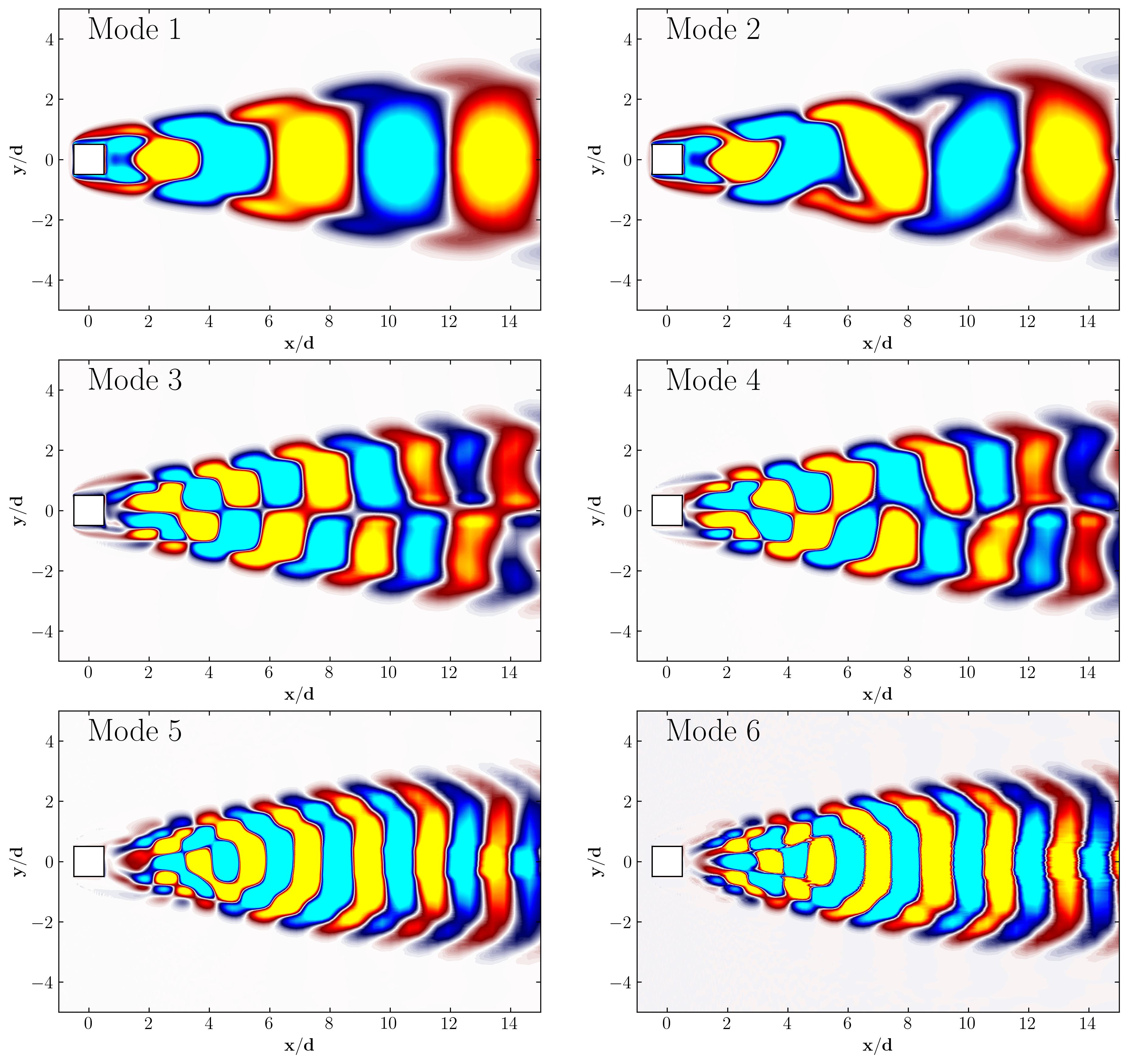
Using this approach, you can plot the first six modes associated with the dominant vortex shedding phenomenon:
Similarly, you can visualize the first six modes corresponding to the second harmonic in the flow:
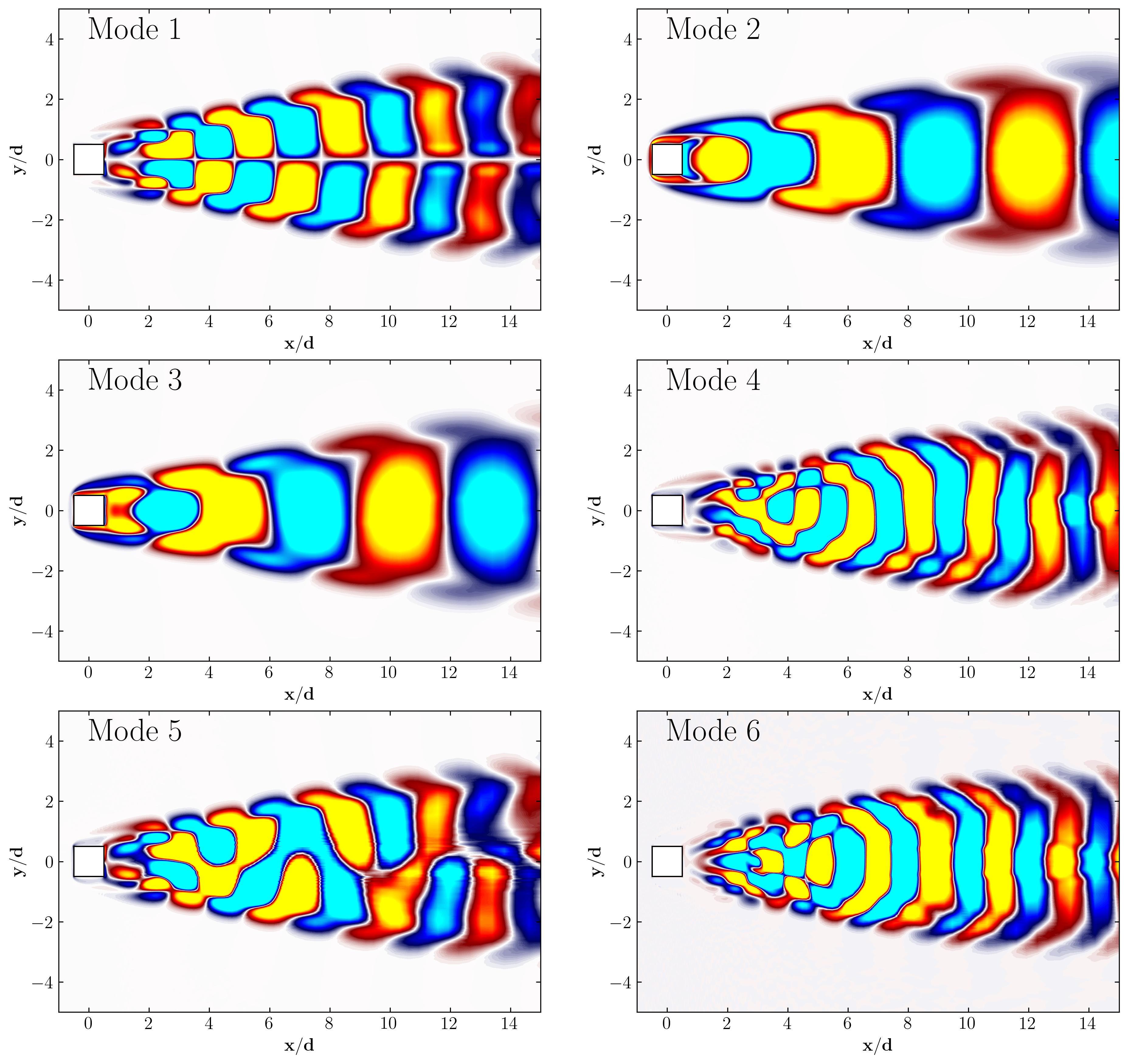
Notice how Mode 1 for both the dominant and second harmonic frequencies closely aligns with POD Modes 1 and 3, which are tied to these specific frequencies:
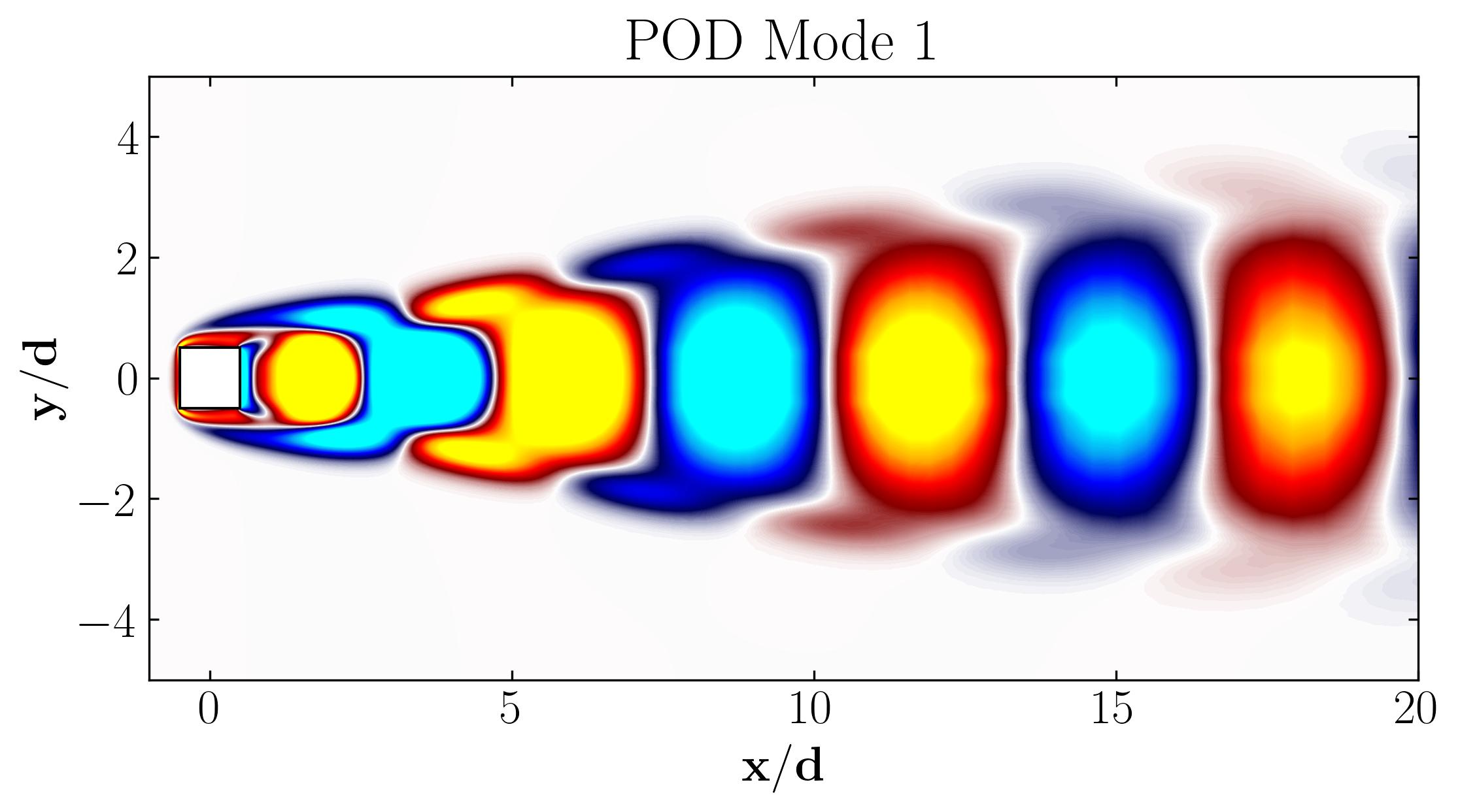
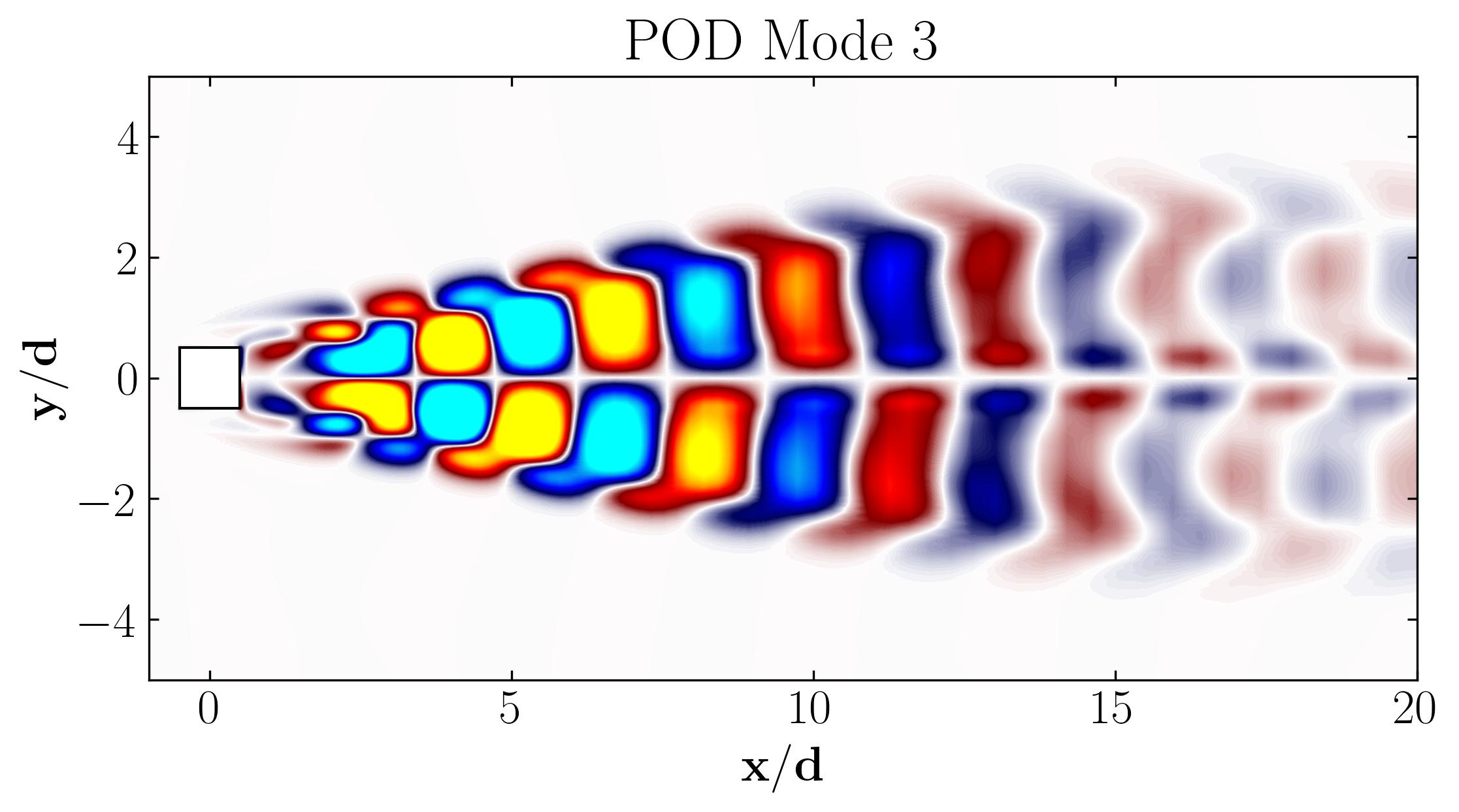
This indicates that the spatial structures identified by SPOD at these frequencies are similar to those captured by POD. This strong correlation suggests that the energy-dominant structures in the dataset (captured by POD) are primarily driven by the dynamics at the dominant frequency and its second harmonic. Understanding the connection between SPOD and POD modes provides valuable insight into the multi-scale nature of the flow or system, revealing how certain modes are prominent across various scales and frequencies.
Enjoy Reading This Article?
Here are some more articles you might like to read next: