Singular Value Decomposition (SVD) is a powerful tool for data analysis, but its output can be overwhelming due to high dimensionality. Optimal Singular Value Hard Thresholding (OSVHT) offers a streamlined approach to address this challenge. By intelligently selecting and retaining only the most significant singular values, OSVHT effectively compresses data while preserving crucial information. This data-driven technique transforms complex datasets into more manageable representations without sacrificing essential insights.

Singular Value Decomposition (SVD) offers a powerful framework for distilling complex, high-dimensional data into a low-dimensional representation that highlights the most significant structures or patterns with precision. The strength of SVD lies in its data-driven nature—requiring no external filters or subjective input—relying purely on the underlying data for insights. However, traditionally, SVD requires expert intervention to determine the optimal rank for dimensionality reduction. This rank selection is often guided by an analyst’s judgment and experience, making it a nuanced task.

Consider for example an $m\times n$ matrix B. Then, SVD of this matrix decomposes B as follows:

The first step in SVD involves examining the singular values contained in the matrix S. These singular values, which are the square roots of the eigenvalues derived from either U or V, are arranged in descending order of magnitude. The expert (you) typically analyzes these values to determine the appropriate rank for dimensionality reduction. Based on this assessment, the expert then truncates the SVD, generating an optimal rank-r approximation of B that best represents the data in a least-squares sense.

But what happens when the expert (you) isn’t available? In scenarios such as automated data processing, is there a way to perform SVD and determine the optimal rank without relying on manual intervention? This challenge prompts the question: can we develop a data-driven, machine learning-based approach to automate the rank selection process from the SVD?

This article introduces the Optimal Singular Value Hard Threshold (OSVHT) method, proposed by Gavish and Donoho (2014). OSVHT provides a systematic, automatic approach to determining the rank, bypassing the need for human judgment while ensuring optimal dimensionality reduction.

Let’s dive in!

The concept

The Optimal Singular Value Hard Threshold (OSVHT) is a method designed to optimize the truncation of singular values, retaining only the most important modes or singular vectors while discarding the rest. OSVHT is particularly useful in matrix denoising and dimensionality reduction tasks, especially when the data can be modeled as a low-rank matrix corrupted by noise. The goal here is to separate the meaningful signal—represented by the low-rank structure—from the noise, which typically manifests as smaller singular values.

In essence, hard thresholding involves setting all singular values below a certain threshold to zero, thus keeping only the dominant singular values that are considered significant. The optimal threshold refers to mathematically determining this cutoff point so that the matrix reconstruction after thresholding minimizes reconstruction error. This allows for an ideal balance between preserving the true low-rank signal and filtering out the noise.

The determination of the OSVHT threshold, denoted as $\tau_\ast$, depends on whether the noise levels are known or unknown. One common assumption is that the noise follows a Gaussian distribution, but in many real-world cases, the noise levels are unknown. When noise is not directly measurable, OSVHT offers methods to estimate the optimal threshold based on the observed data.

Where $\beta = m/n$ (with $m \leq n$), $y_{med}$ is the median singular value of the data matrix B, and $\omega(\beta)$ can be approximated by the following formula:

Note that the exact computation of $\omega(\beta)$ is possible by evaluating the median of the Marchenko-Pastur distribution, denoted $\mu_\beta$, such that:

Here, $\lambda_\ast(\beta)$ is the critical value associated with the Marchenko-Pastur distribution.

In this way, the OSVHT threshold, denoted $\tau_\ast$, provides a single value that represents the optimal rank for dimensionality reduction. This threshold effectively separates the true modes (representing the signal) from the noisy, irrelevant modes. Once the optimal SVHT is applied, you can truncate the SVD and reconstruct a de-noised version of the data matrix. The new matrix retains the essential structure but without the noise!

Python Implementation

Let’s now explore the Python implementation of the Optimal Singular Value Hard Threshold (OSVHT) method. We’ll start by importing the necessary modules:

import numpy as np
import matplotlib.pyplot as plt
import scipy as sp
%matplotlib inline
plt.rcParams.update({'font.size' : 14, 'font.family' : 'Times New Roman', "text.usetex": True})
savePath = 'E:/Blog_Posts/OpenFOAM/ROM_Series/Post35/'

Next, we generate a noisy data matrix:

x = np.linspace(-10, 10, 100)
t = np.linspace(0, 20, 200)
Xm, Tm = np.meshgrid(x, t)

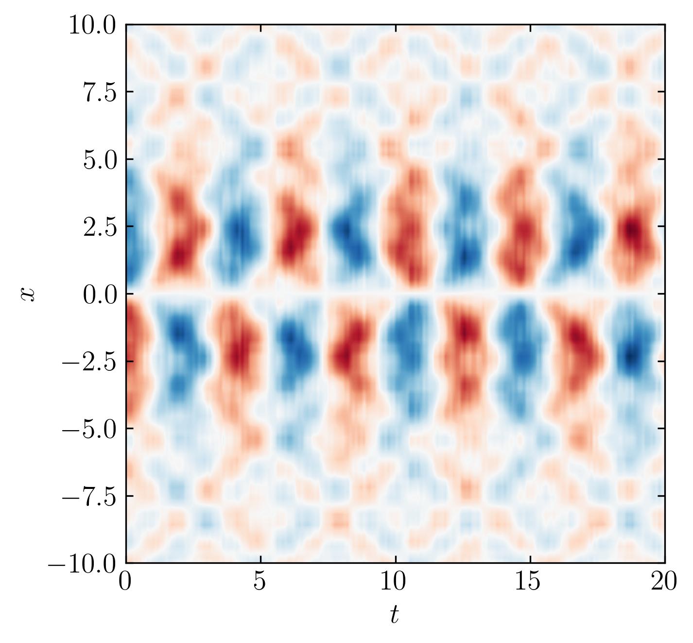
data_matrix = 5.0 / np.cosh(0.5*Xm) * np.tanh(0.5*Xm) * np.exp(1.5j*Tm) # primary mode
data_matrix += 0.5 * np.sin(2.0*Xm) * np.exp(2.0j*Tm) # secondary mode
data_matrix += 0.5 * np.sin(3.2*Xm) * np.cosh(3.2j*Tm) # tertiary mode
data_matrix += 0.5 * np.random.randn(Xm.shape[0], Tm.shape[1]) # noise

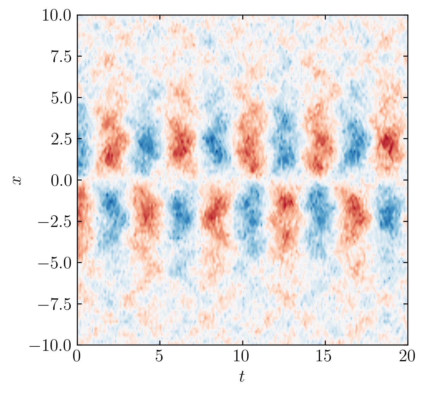
This generates a synthetic dataset with three distinct modes and random noise added to simulate real-world conditions.

The Python functions for calculating the median of the Marchenko-Pastur distribution and $\lambda_\ast$ (Lambda Star) are as follows:

def mar_pas(x, topSpec, botSpec, beta):
    """Implement Marcenko-Pastur distribution."""
    if (topSpec - x) * (x - botSpec) > 0:
        return np.sqrt((topSpec - x) *
                       (x - botSpec)) / (beta * x) / (2 * np.pi)
    else:
        return 0


def median_marcenko_pastur(beta):
    """Compute median of Marcenko-Pastur distribution."""
    botSpec = lobnd = (1 - np.sqrt(beta))**2
    topSpec = hibnd = (1 + np.sqrt(beta))**2
    change = 1

    while change & ((hibnd - lobnd) > .001):
        change = 0
        x = np.linspace(lobnd, hibnd, 10)
        y = np.zeros_like(x)
        for i in range(len(x)):
            yi, err = sp.integrate.quad(
                mar_pas,
                a=x[i],
                b=topSpec,
                args=(topSpec, botSpec, beta),
            )
            y[i] = 1.0 - yi

        if np.any(y < 0.5):
            lobnd = np.max(x[y < 0.5])
            change = 1

        if np.any(y > 0.5):
            hibnd = np.min(x[y > 0.5])
            change = 1

    return (hibnd + lobnd) / 2.

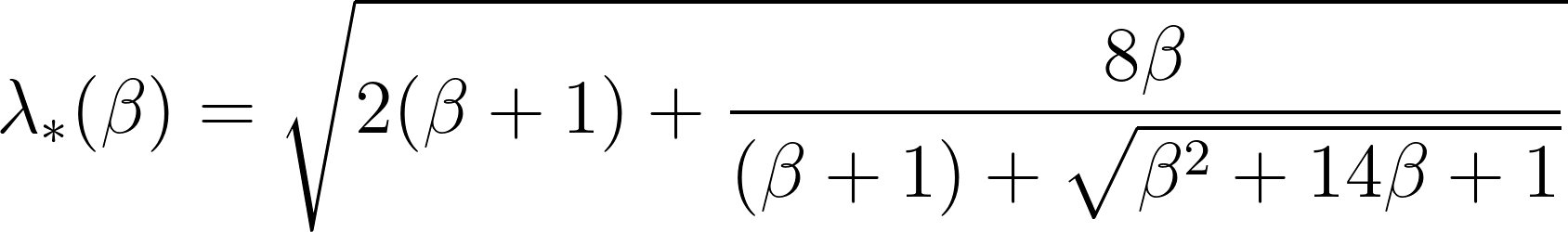
def lambda_star(beta):
    """Return lambda star for given beta. Equation (11) from Gavish 2014."""
    return np.sqrt(2 * (beta + 1) + (8 * beta) / 
                   (beta + 1 + np.sqrt(beta**2 + 14 * beta + 1)))

Now, let’s perform the SVD on the noisy data matrix:

U, s, Vh = np.linalg.svd(data_matrix, full_matrices=False)

Next, we compute the Optimal Singular Value Hard Threshold (OSVHT) as follows:

Omega_beta = lambda_star(beta)/np.sqrt(median_marcenko_pastur(beta))
tau = Omega_beta * np.median(s)

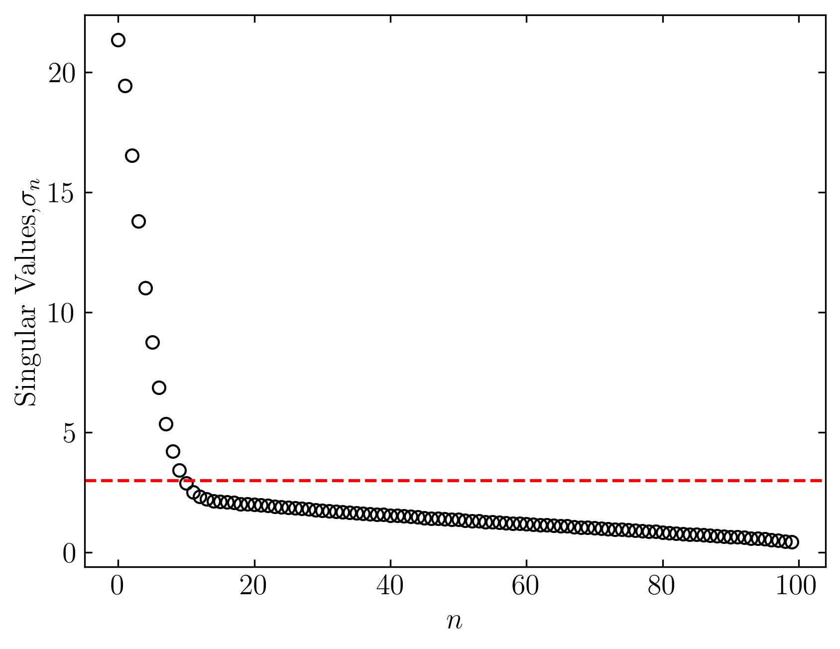
To visualize the result, let’s plot the singular values of the data matrix:

fig, ax = plt.subplots()

ax.plot(s, marker = 'o', markerfacecolor = 'none', markeredgecolor = 'k', ls='', color = 'k')
ax.axhline(y = tau, color = 'r', ls = '--')

ax.set_xlabel(r'$n$')
ax.set_ylabel('Singular Values,' + r'$\sigma_n$')
ax.xaxis.set_tick_params(direction='in', which='both')
ax.yaxis.set_tick_params(direction='in', which='both')
ax.xaxis.set_ticks_position('both')
ax.yaxis.set_ticks_position('both')
plt.show()

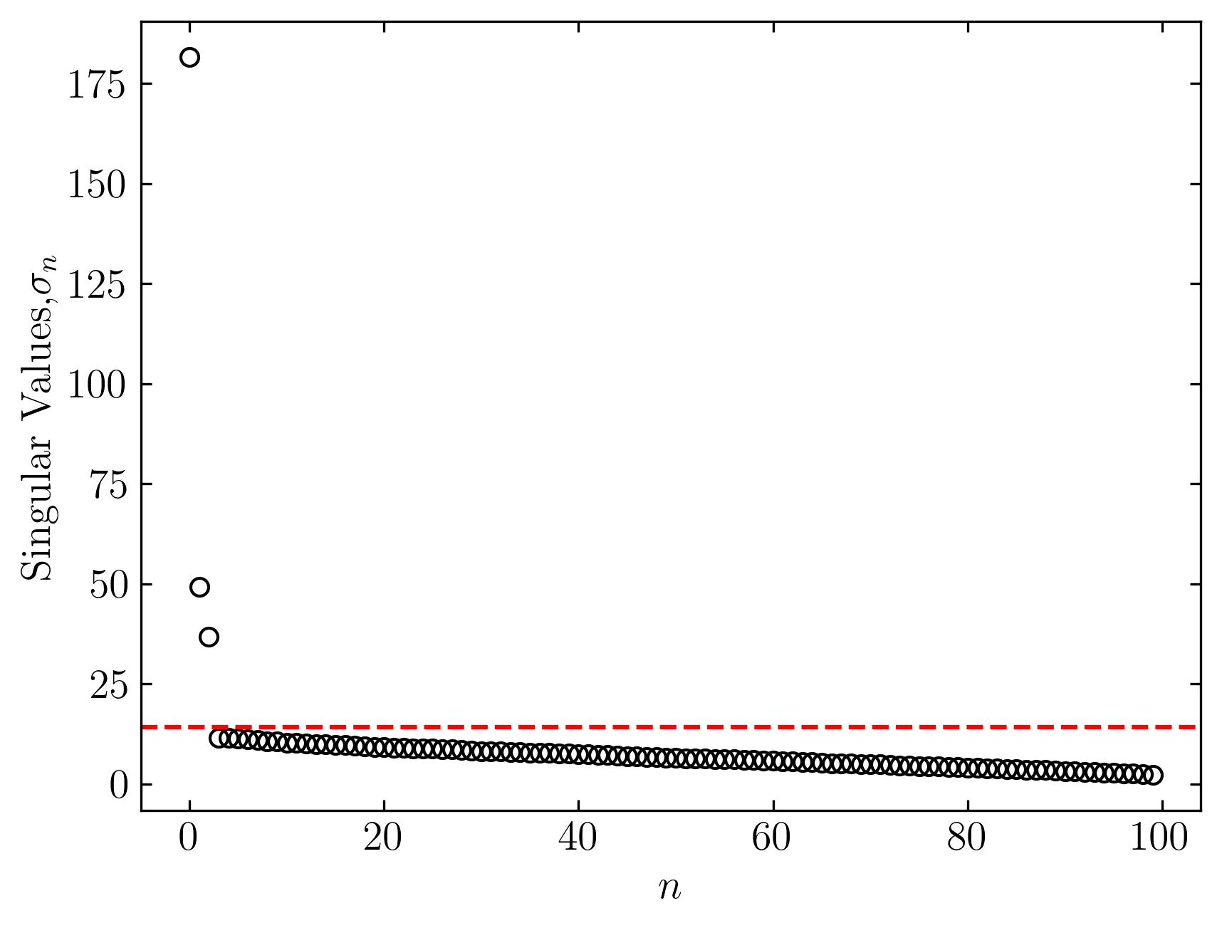
In this plot, the red dashed line represents the optimal truncation threshold. Notice how this method effectively separates the largest and most dominant singular values from the smaller ones, which typically represent noise.

Finally, let’s truncate the SVD and reconstruct the data to produce the de-noised version:

s2 = s.copy()
s2[s < tau] = 0
D2 = np.dot(np.dot(U, np.diag(s2)), Vh)

fig, ax = plt.subplots()
p = ax.contourf(t, x, D2.T, levels = 501, cmap = 'RdBu')
ax.xaxis.set_tick_params(direction='in', which='both')
ax.yaxis.set_tick_params(direction='in', which='both')
ax.xaxis.set_ticks_position('both')
ax.yaxis.set_ticks_position('both')
ax.set_aspect('equal')
ax.set_xlabel(r'$t$')
ax.set_ylabel(r'$x$')

plt.show()

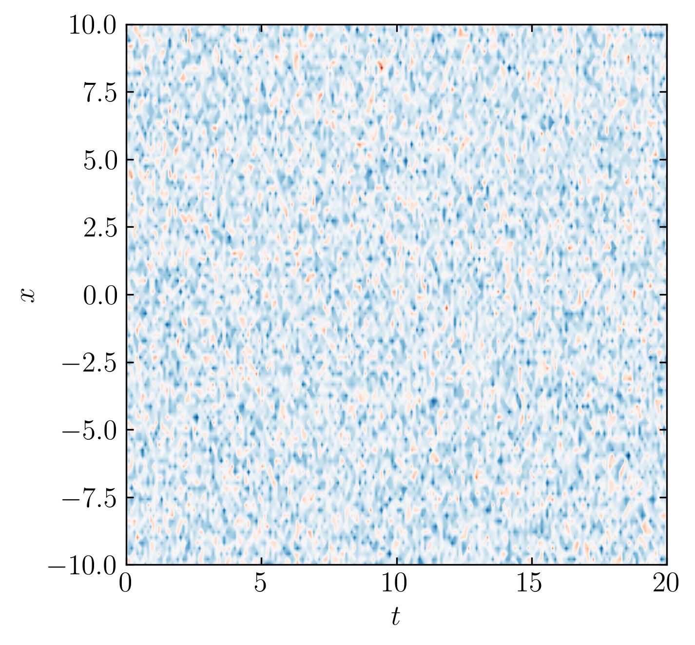
Random Data

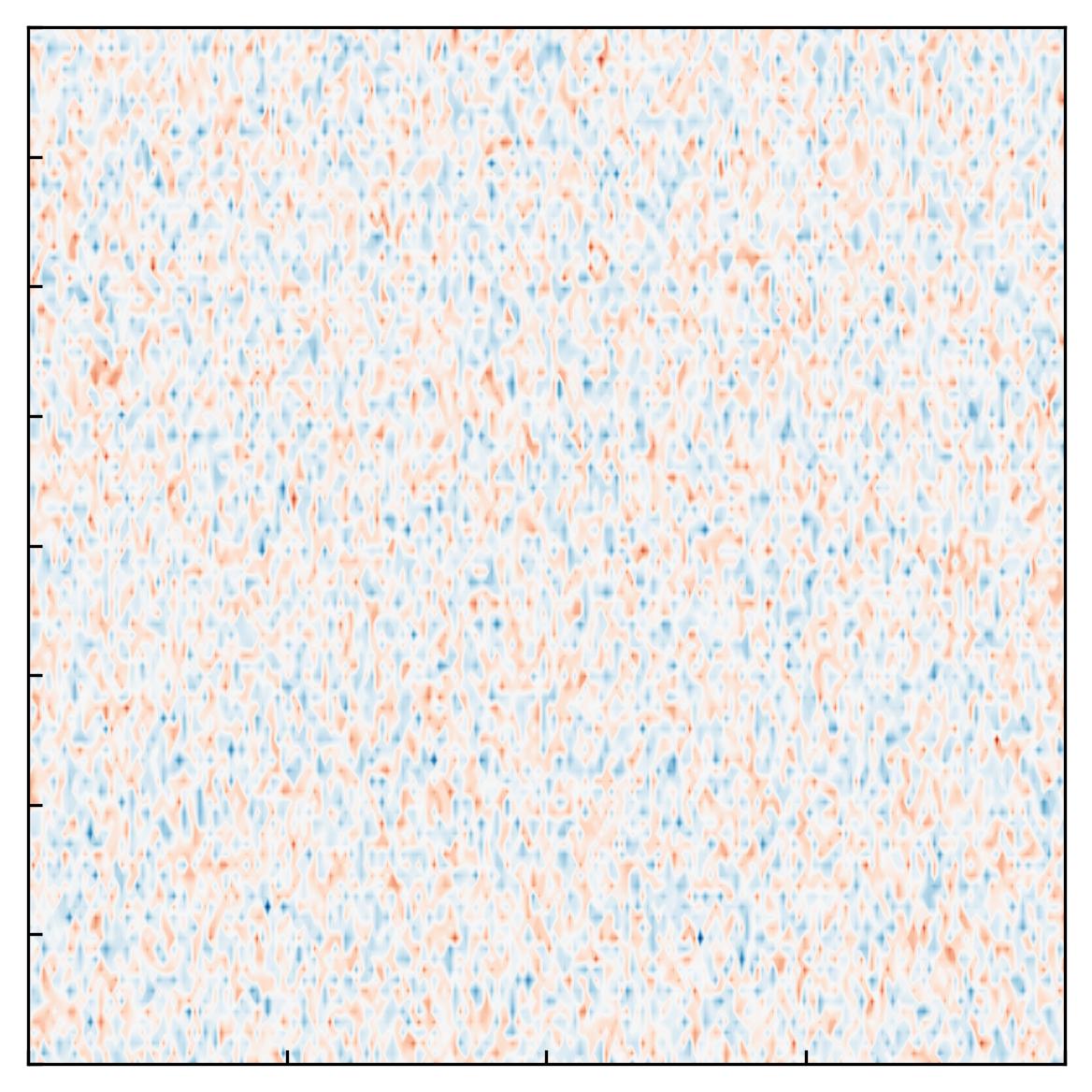
To validate the effectiveness of the code, let’s test it on a completely random dataset. Ideally, for a purely random dataset, the Optimal Singular Value Hard Threshold (OSVHT) should suggest truncating the entire dataset, as there would be no meaningful signal present. Let’s explore this hypothesis by generating a completely random dataset:

CRD = np.random.randn(n, m)

fig, ax = plt.subplots()

p = ax.contourf(t, x, CRD.T, levels = 501, cmap = 'RdBu')
ax.xaxis.set_tick_params(direction='in', which='both')
ax.yaxis.set_tick_params(direction='in', which='both')
ax.xaxis.set_ticks_position('both')
ax.yaxis.set_ticks_position('both')
ax.set_aspect('equal')

ax.set_xlabel(r'$t$')
ax.set_ylabel(r'$x$')
plt.show()

Then calculate the SVD and OSVHT:

U, s, Vh = np.linalg.svd(CRD, full_matrices=False)
tau = Omega_beta * np.median(s)

fig, ax = plt.subplots()

ax.plot(s, marker = 'o', markerfacecolor = 'none', markeredgecolor = 'k', ls='', color = 'k')
ax.axhline(y = tau, color = 'r', ls = '--')

ax.set_xlabel(r'$n$')
ax.set_ylabel('Singular Values,' + r'$\sigma_n$')
ax.xaxis.set_tick_params(direction='in', which='both')
ax.yaxis.set_tick_params(direction='in', which='both')
ax.xaxis.set_ticks_position('both')
ax.yaxis.set_ticks_position('both')
plt.show()

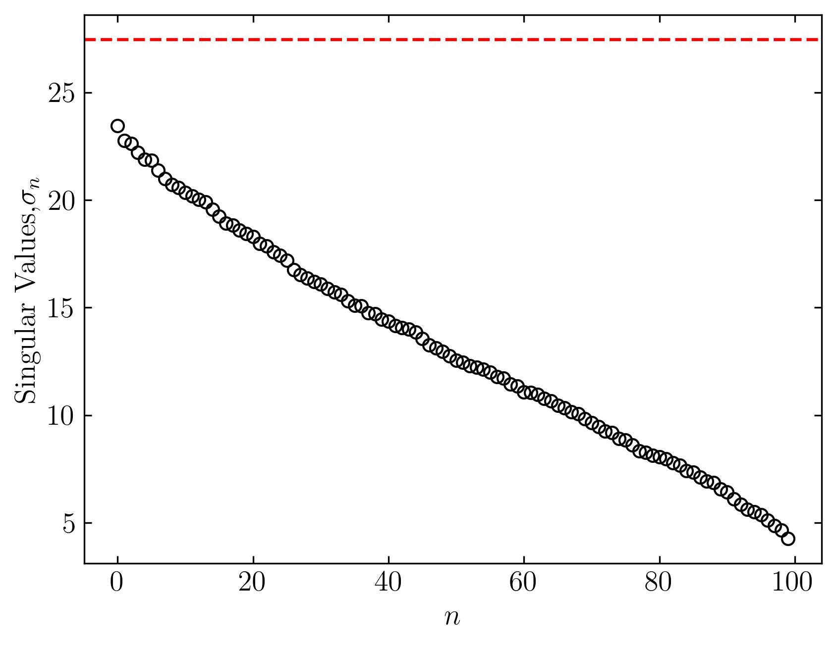
It works!!!

Translational Invariance

Translational invariance is a special case where the data may be inherently low-dimensional, yet the SVD might misleadingly indicate high-dimensionality. Let’s see if OSVHT can effectively handle this scenario.

def sech(x):
    return 1/np.cosh(x)

BT = sech(Xm + 6 - Tm) * np.exp(2.3j*Tm) # primary mode
BT += 0.1 * np.random.randn(Xm.shape[0], Tm.shape[1])

fig, ax = plt.subplots()
p = ax.contourf(t, x, BT.T, levels = 501, cmap = 'RdBu')
ax.xaxis.set_tick_params(direction='in', which='both')
ax.yaxis.set_tick_params(direction='in', which='both')
ax.xaxis.set_ticks_position('both')
ax.yaxis.set_ticks_position('both')
ax.set_aspect('equal')
ax.set_xlabel(r'$t$')
ax.set_ylabel(r'$x$')
plt.show()

Perform SVD and OSVHT on this data:

U, s, Vh = np.linalg.svd(BT, full_matrices=False)
tau = Omega_beta * np.median(s)

fig, ax = plt.subplots()

ax.plot(s, marker = 'o', markerfacecolor = 'none', markeredgecolor = 'k', ls='', color = 'k')
ax.axhline(y = tau, color = 'r', ls = '--')

ax.set_xlabel(r'$n$')
ax.set_ylabel('Singular Values,' + r'$\sigma_n$')
ax.xaxis.set_tick_params(direction='in', which='both')
ax.yaxis.set_tick_params(direction='in', which='both')
ax.xaxis.set_ticks_position('both')
ax.yaxis.set_ticks_position('both')

plt.show()

Check the low-rank reconstruction:

s2 = s.copy()
s2[s < tau] = 0
D2 = np.dot(np.dot(U, np.diag(s2)), Vh)

fig, ax = plt.subplots()

p = ax.contourf(t, x, D2.T, levels = 501, cmap = 'RdBu')
ax.xaxis.set_tick_params(direction='in', which='both')
ax.yaxis.set_tick_params(direction='in', which='both')
ax.xaxis.set_ticks_position('both')
ax.yaxis.set_ticks_position('both')
ax.set_aspect('equal')
ax.set_xlabel(r'$t$')
ax.set_ylabel(r'$x$')
plt.show()

It works!!! The optimal SVHT still recommends a sensible rank for row-reduction.

Overall, the OSVHT method offers a valuable tool for improving data analysis and reconstruction in various applications, making it a worthy addition to the toolkit of anyone working with high-dimensional data.