Sparsity Promoting Dynamic Mode Decomposition: A Game Changer in Data-Driven Analysis
In the world of data-driven analysis, extracting meaningful patterns from complex fluid flows is a significant challenge. Sparsity Promoting Dynamic Mode Decomposition (SPDMD) offers a powerful approach to uncovering the most dominant features while discarding redundant information, leading to a more efficient and insightful decomposition. This method blends the mathematical elegance of Dynamic Mode Decomposition (DMD) with sparse optimization techniques, providing a robust framework to identify critical structures in high-dimensional data.
Dynamic Mode Decomposition (DMD) has become a cornerstone of data-driven modeling in fluid dynamics, providing a powerful means to break down complex, high-dimensional flow data into fundamental spatiotemporal modes. However, standard DMD methods face several limitations, particularly in handling translational invariances and transient phenomena. Check out my previous article on DMD and its limitations here. These limitations highlight the importance of extending DMD methodologies to more sophisticated versions, ones that tweak the DMD algorithm such that these limitations can be overcome. In this article, Lets explore one such variant of DMD names Sparsity-promoting Dynamic Mode Decomposition.
Standard DMD often generate an excessive number of modes, many of which are redundant or heavily influenced by noise, making it challenging to pinpoint the essential flow dynamics. This lack of selectivity can obscure important features and complicate the interpretation of results, particularly in cases involving large datasets or systems with high noise levels. Sparsity Promoting Dynamic Mode Decomposition (SPDMD) was developed by Jovanovic et al. (2014) to address these challenges. By integrating sparse optimization techniques, SPDMD selectively retains only the most significant modes, effectively filtering out the less relevant ones. This enhances the clarity and interpretability of the decomposition, leading to a more concise representation of the underlying physics. The sparsity constraint also reduces computational costs, making SPDMD particularly suitable for real-time applications and large-scale simulations.
This approach has shown great promise in various applications, such as identifying coherent structures in turbulent flows, detecting wake vortices in aerodynamics, and uncovering dominant patterns in environmental monitoring datasets. For instance, in studying wake flows behind bluff bodies, SPDMD has been able to isolate the most critical vortical structures responsible for energy transfer, offering deeper insights into the wake dynamics than traditional DMD methods. Similarly, in climate science, SPDMD has helped identify key modes of variability in ocean currents and atmospheric patterns, improving the understanding of large-scale environmental phenomena.
In this blog, lets understand the fundamentals of SPDMD using a toy example and python to revolutionize data-driven analysis in fluid dynamics and beyond. Lets begin!!
Sparsity-Promoting DMD
The key idea behind Sparsity-Promoting Dynamic Mode Decomposition (SPDMD) is straightforward: How can we find the most representative DMD modes to capture the essential dynamics of a system? While this question may seem simple, it is more profound than one might initially think. Traditionally, Dynamic Mode Decomposition (DMD) is performed by a human expert who carefully selects the DMD modes based on their experience and understanding of the data. But what happens when we want to automate this process, removing the need for human intervention?
This is where SPDMD comes into play. Similar to how methods like the Optimal Singular Value Hard Threshold (OSVHT) provide an automated approach for Singular Value Decomposition (SVD), SPDMD offers a way to automate the selection of DMD modes. SPDMD leverages an optimization algorithm to redefine the calculation of mode amplitudes in DMD, aiming to reconstruct the original dataset using the fewest possible modes. The goal is to extract the most critical dynamics of the system. The term “sparsity-promoting” refers to the preference for solutions with a minimal number of nonzero modes, focusing on the most impactful dynamic features.
Building upon the classical DMD framework, SPDMD introduces a sparsity constraint that selectively identifies the most important dynamic modes. The process begins similarly to traditional DMD: given a sequence of snapshots (time-series data) from a fluid flow or another dynamical system, DMD seeks a low-rank approximation of the data by decomposing it into spatial modes, each characterized by its temporal evolution through an eigenvalue.
The innovation of SPDMD lies in its use of a sparsity-promoting optimization technique, typically incorporating an $L_1$-norm regularization term. Unlike the $L_2$-norm used in traditional methods, the $L_1$-norm encourages sparsity by penalizing the number of non-zero entries. In the context of DMD, this approach allows the optimization algorithm to identify a minimal subset of modes that best represent the system’s dynamics, minimizing the influence of less significant or redundant modes.
For a comprehensive overview of the mathematics behind Dynamic Mode Decomposition (DMD), please refer to my previous article.
Recall that the DMD mode amplitudes are given by:
\[b = \Phi^\dagger x_1\]Where, $\Phi$ represent the DMD modes, defined as:
\[\Phi = UW\]The optimization problem for SPDMD can be mathematically formulated as:
\[\min_{b} ||X - \Phi diag(b)V^\ast||_F^2 + \lambda ||b||_1\]where:
- $X$ is the matrix containing the snapshot data,
- $\Phi$ is the matrix of DMD modes,
- $b$ is a vector of mode amplitudes,
- $\lambda$ is a sparsity parameter controlling the balance between reconstruction accuracy and sparsity.
By adjusting the parameter $\lambda$, SPDMD determines how many modes are retained, enabling a more compact representation of the data. As $\lambda$ increases, the method promotes greater sparsity, resulting in fewer selected modes. This yields a clearer and more interpretable set of modes that capture the most dominant and physically meaningful features of the system.
To solve this optimization problem, SPDMD employs the Alternating Direction Method of Multipliers (ADMM) algorithm. ADMM is particularly effective for problems with large datasets, constraints, or regularization terms that promote sparsity. It iteratively searches for the optimal mode amplitude vector $b$ that minimizes the cost function while ensuring the vector is sparse, containing very few non-zero entries.
Toy Example
To illustrate the concept of SPDMD, let’s explore a toy example. We will begin by loading the necessary modules into a Jupyter notebook:
import matplotlib.colors
import matplotlib.pyplot as plt
import numpy as np
import pandas as pd
import scipy as sp
from matplotlib.colors import ListedColormap
import os
import io
%matplotlib inline
plt.rcParams.update({'font.size' : 18, 'font.family' : 'Times New Roman', "text.usetex": True})

savePath = 'E:/Blog_Posts/OpenFOAM/ROM_Series/Post36/'
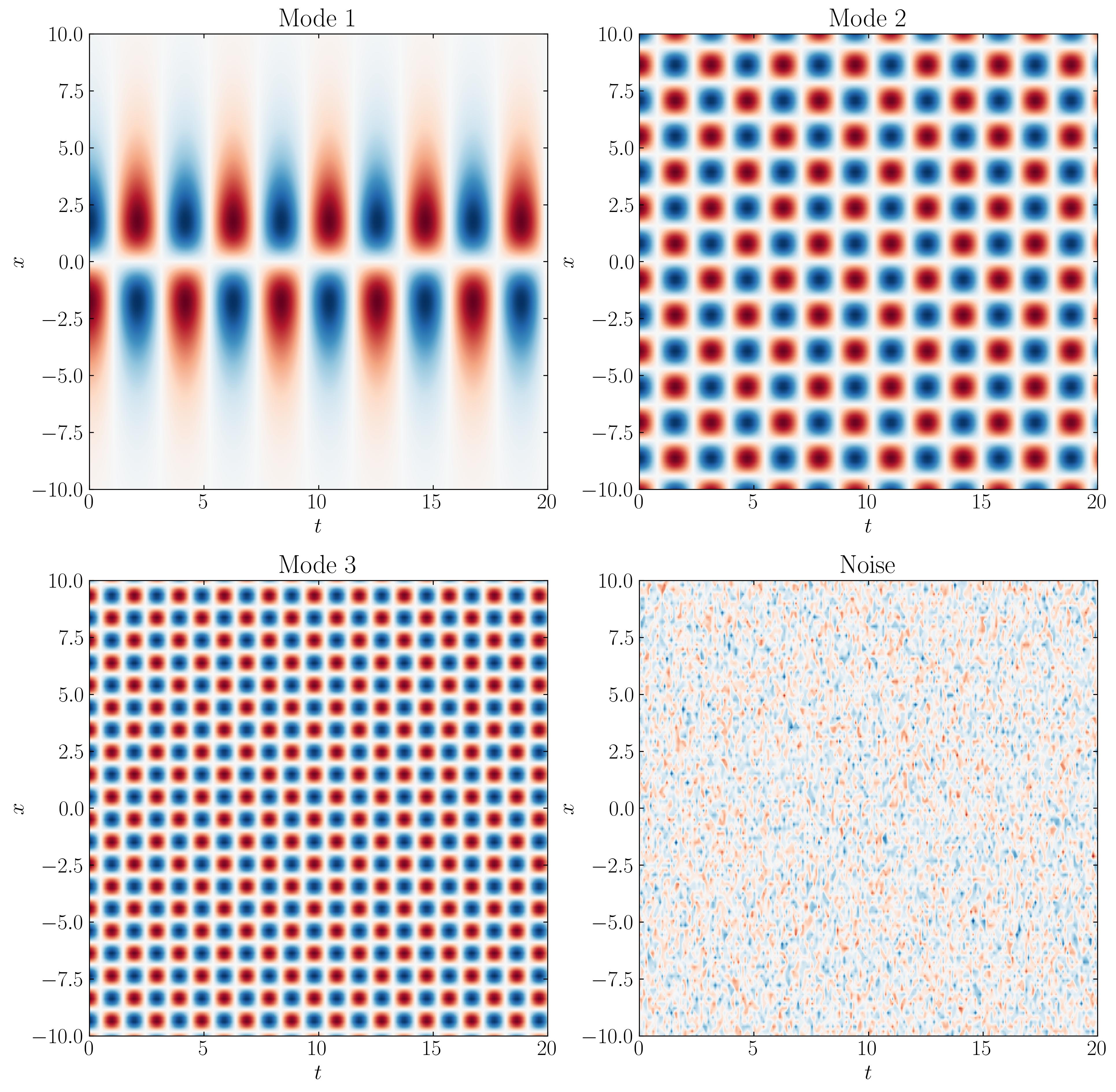
Next, let’s generate a toy signal consisting of three distinct modes and some added noise. The resulting data will be mean-removed and normalized to better illustrate the dynamics captured by SPDMD.
x = np.linspace(-10, 10, 100)
t = np.linspace(0, 20, 200)
Xm, Tm = np.meshgrid(x, t)

M1 = 5.0 / np.cosh(0.5*Xm) * np.tanh(0.5*Xm) * np.exp(1.5j*Tm) # primary mode
M2 = 0.5 * np.sin(2.0*Xm) * np.exp(2.0j*Tm) # secondary mode
M3 = 0.5 * np.sin(3.2*Xm) * np.cosh(3.2j*Tm) # tertiary mode
M4 = 0.5 * np.random.randn(Xm.shape[0], Tm.shape[1]) # noise

data_matrix = M1 + M2 + M3 + M4
You can visualize the three modes and the noise as follows:
d = 0.1
Ub = 0.015

fig, axs = plt.subplots(2, 2, figsize=(15, 15))

ax = axs[0,0]
p = ax.contourf(t, x, M1.T, levels = 501, cmap = 'RdBu')
ax.xaxis.set_tick_params(direction='in', which='both')
ax.yaxis.set_tick_params(direction='in', which='both')
ax.xaxis.set_ticks_position('both')
ax.yaxis.set_ticks_position('both')

ax.set_ylabel(r'$x$')
ax.set_xlabel(r'$t$')
ax.set_title('Mode 1')

ax = axs[0,1]
p = ax.contourf(t, x, M2.T, levels = 501, cmap = 'RdBu')
ax.xaxis.set_tick_params(direction='in', which='both')
ax.yaxis.set_tick_params(direction='in', which='both')
ax.xaxis.set_ticks_position('both')
ax.yaxis.set_ticks_position('both')

ax.set_ylabel(r'$x$')
ax.set_xlabel(r'$t$')
ax.set_title('Mode 2')

ax = axs[1,0]
p = ax.contourf(t, x, M3.T, levels = 501, cmap = 'RdBu')
ax.xaxis.set_tick_params(direction='in', which='both')
ax.yaxis.set_tick_params(direction='in', which='both')
ax.xaxis.set_ticks_position('both')
ax.yaxis.set_ticks_position('both')

ax.set_ylabel(r'$x$')
ax.set_xlabel(r'$t$')
ax.set_title('Mode 3')

ax = axs[1,1]
p = ax.contourf(t, x, M4.T, levels = 501, cmap = 'RdBu')
ax.xaxis.set_tick_params(direction='in', which='both')
ax.yaxis.set_tick_params(direction='in', which='both')
ax.xaxis.set_ticks_position('both')
ax.yaxis.set_ticks_position('both')

ax.set_ylabel(r'$x$')
ax.set_xlabel(r'$t$')
ax.set_title('Noise')

plt.show()
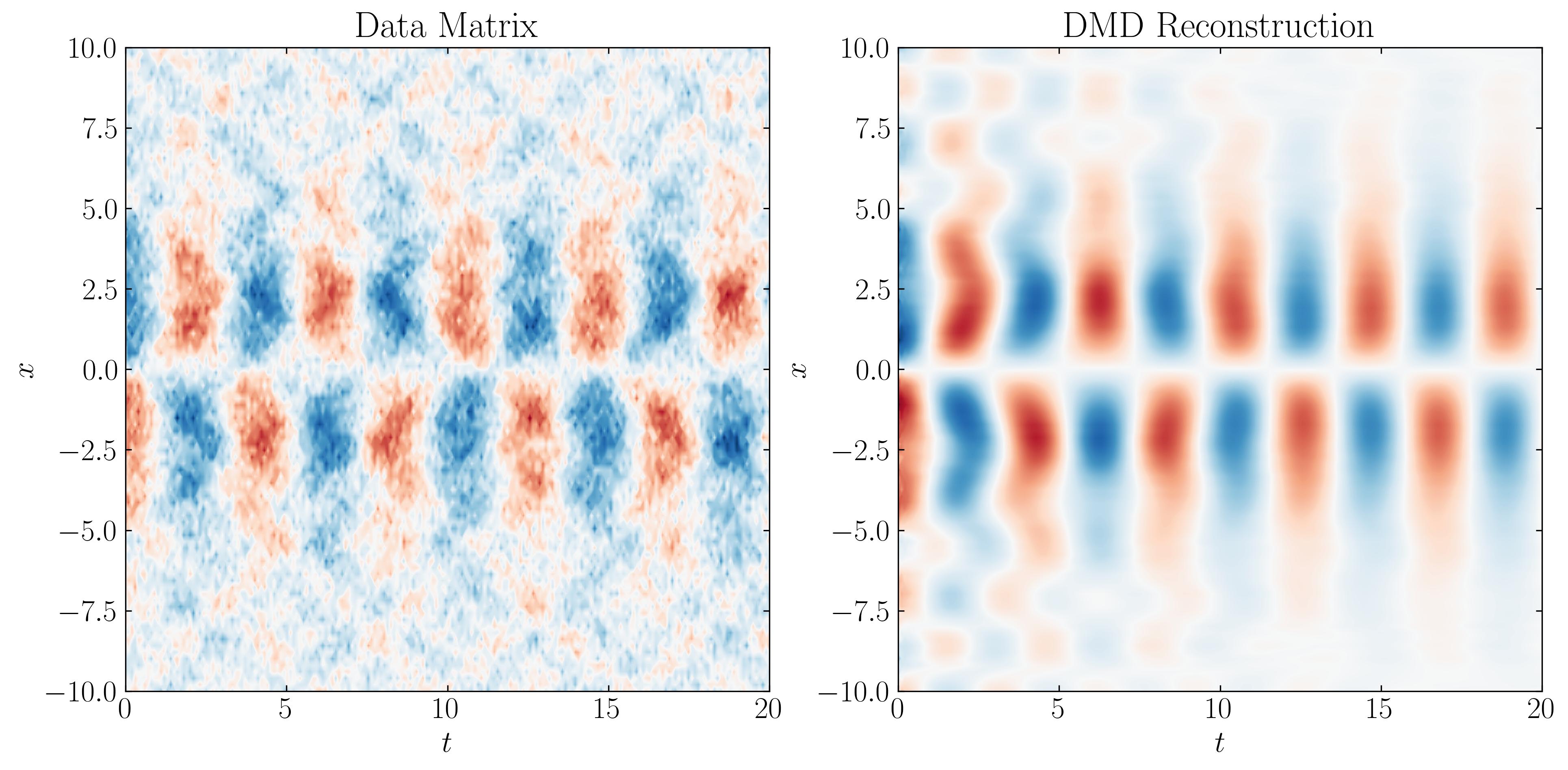
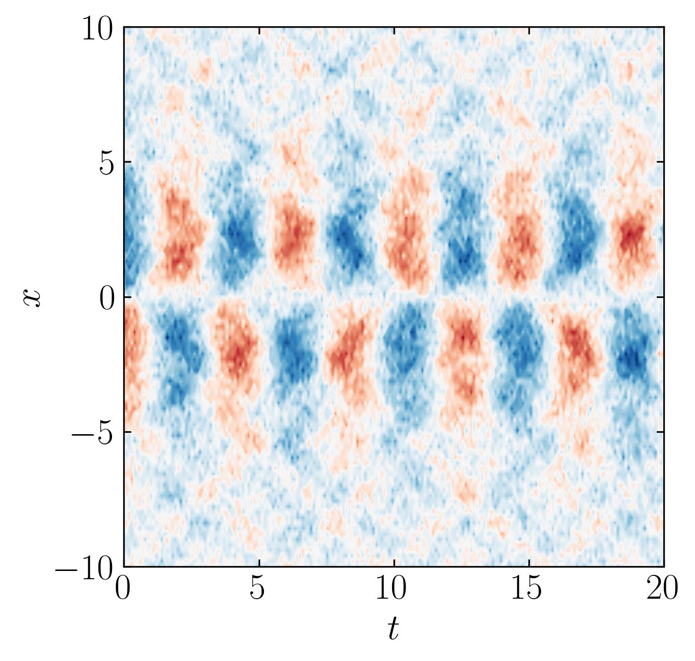
The combination of these three modes, along with the added noise, forms the data matrix that we will input into the DMD algorithm. This data matrix appears as follows:
The algorithm for standard Dynamic Mode Decomposition (DMD) is as follows:
def DMD(X1, X2, r, dt):
    U, s, Vh = np.linalg.svd(X1, full_matrices=False)
    ### Truncate the SVD matrices
    Ur = U[:, :r]
    Sr = np.diag(s[:r])
    Vr = Vh.conj().T[:, :r]

    ### Build the Atilde and find the eigenvalues and eigenvectors
    Atilde = Ur.conj().T @ X2 @ Vr @ np.linalg.inv(Sr)
    Lambda, W = np.linalg.eig(Atilde)

    ### Compute the DMD modes
    Phi = X2 @ Vr @ np.linalg.inv(Sr) @ W

    omega = np.log(Lambda)/dt ### continuous time eigenvalues

    ### Compute the amplitudes

    alpha1 = np.linalg.lstsq(Phi, X1[:, 0], rcond=None)[0] ### DMD mode amplitudes

    b = np.linalg.lstsq(Phi, X2[:, 0], rcond=None)[0] ### DMD mode amplitudes

    return Phi, omega, Lambda, alpha1, b
Now, let’s pass the data matrix into the above DMD algorithm:
# Time shifted snapshot matrix
X1 = data_matrix.T[:, :-1]
X2 = data_matrix.T[:, 1:]

r = 30 # Rank of truncation
dt = t[1] - t[0]

# DMD
Phi, omega, Lambda, alpha1, b = DMD(X1, X2, r, dt)
The next step in the DMD workflow is to reconstruct a matrix representing the time evolution of the system. To do this, we compute the time dynamics and obtain the DMD reconstruction:
\[X_{DMD} = \Phi \cdot \Psi\]Typically, the system’s initial conditions at $x_0$ are used to create a time evolution matrix. However, we will use an alternative formulation that leverages a Vandermonde matrix:
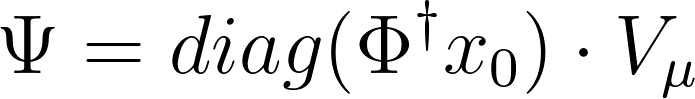
Where, $V_\mu$ is the Vandermonde matrix and $\dagger$ is the Moore-Penrose pseudo-inverse of a matrix.
# compute time evolution (concise way)
Vand = np.vander(Lambda, len(t), True)
Psi = (Vand.T * b).T # equivalently, Psi = dot(diag(b), Vand)
We can then reconstruct the reduced-order approximation of the data as follows:
D_dmd = np.dot(Phi, Psi) # reconstruct data

The Catch
Now, here’s the catch: we are not restricted to using the initial conditions ($x_0$) of the system to construct the amplitude vector b, traditionally defined as:
$b = \Phi^\dagger x_0$
Instead, we can potentially choose b to be a vector that produces a time evolution even closer to the original data by minimizing the reconstruction error. This allows us to redefine the DMD mode amplitudes by minimizing the following objective:

To simplify the first term, we can use the matrix trace properties, as detailed in Jovanovic et al. (2014):
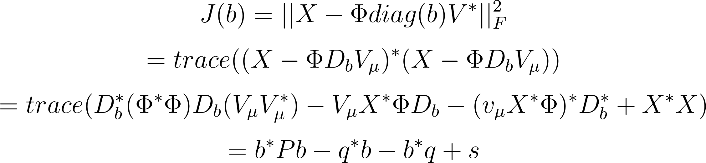
where:
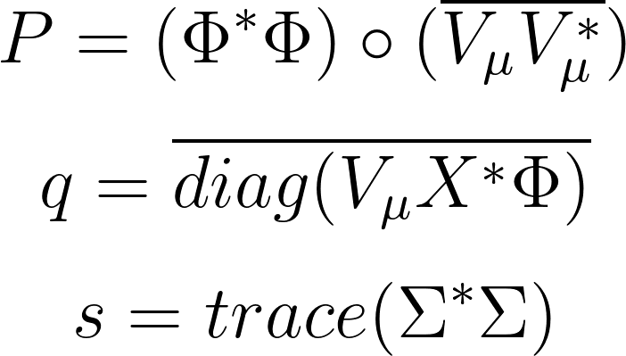
To promote sparsity in the vector b, we introduce an $L_1$ penalty. The purpose of this penalty is to encourage a sparse b vector, containing very few non-zero entries. This optimization is performed using the Alternating Direction Method of Multipliers (ADMM) algorithm. The ADMM code provided below is a direct translation of the MATLAB code used by Jovanovic et al. (2014).
from numpy import dot, multiply, diag
from numpy.linalg import inv, eig, pinv, norm, solve, cholesky
from scipy.linalg import svd, svdvals
from scipy.sparse import csc_matrix as sparse
from scipy.sparse import vstack as spvstack
from scipy.sparse import hstack as sphstack
from scipy.sparse.linalg import spsolve

def admm_for_dmd(P, q, s, gamma_vec, rho=1, maxiter=1000, eps_abs=1e-6, eps_rel=1e-4):

    # blank return value
    answer = type('ADMMAnswer', (object,), {})()

    # check input vars
    P = np.squeeze(P)
    q = np.squeeze(q)[:,np.newaxis]
    gamma_vec = np.squeeze(gamma_vec)
    if P.ndim != 2:
        raise ValueError('invalid P')
    if q.ndim != 2:
        raise ValueError('invalid q')
    if gamma_vec.ndim != 1:
        raise ValueError('invalid gamma_vec')

    # number of optimization variables
    n = len(q)

    # identity matrix
    I = np.eye(n)

    # allocate memory for gamma-dependent output variables
    answer.gamma = gamma_vec
    answer.Nz    = np.zeros([len(gamma_vec),]) # number of non-zero amplitudes
    answer.Jsp   = np.zeros([len(gamma_vec),]) # square of Frobenius norm (before polishing)
    answer.Jpol  = np.zeros([len(gamma_vec),]) # square of Frobenius norm (after polishing)
    answer.Ploss = np.zeros([len(gamma_vec),]) # optimal performance loss (after polishing)
    answer.xsp   = np.zeros([n, len(gamma_vec)], dtype='complex') # vector of amplitudes (before polishing)
    answer.xpol  = np.zeros([n, len(gamma_vec)], dtype='complex') # vector of amplitudes (after polishing)

    # Cholesky factorization of matrix P + (rho/2)*I
    Prho = P + (rho/2) * I
    Plow = cholesky(Prho)
    Plow_star = Plow.conj().T

    # sparse P (for KKT system)
    Psparse = sparse(P)

    for i,gamma in enumerate(gamma_vec):

        # initial conditions
        y = np.zeros([n, 1], dtype='complex') # Lagrange multiplier
        z = np.zeros([n, 1], dtype='complex') # copy of x

        # Use ADMM to solve the gamma-parameterized problem
        for step in range(maxiter):

            # x-minimization step
            u = z - (1/rho) * y
            # x = solve((P + (rho/2) * I), (q + rho * u))
            xnew = solve(Plow_star, solve(Plow, q + (rho/2) * u))

            # z-minimization step
            a = (gamma/rho) * np.ones([n, 1])
            v = xnew + (1/rho) * y
            # soft-thresholding of v
            znew = multiply(multiply(np.divide(1 - a, np.abs(v)), v), (np.abs(v) > a))

            # primal and dual residuals
            res_prim = norm(xnew - znew, 2)
            res_dual = rho * norm(znew - z, 2)

            # Lagrange multiplier update step
            y += rho * (xnew - znew)

            # stopping criteria
            eps_prim = np.sqrt(n) * eps_abs + eps_rel * np.max([norm(xnew, 2), norm(znew, 2)])
            eps_dual = np.sqrt(n) * eps_abs + eps_rel * norm(y, 2)

            if (res_prim < eps_prim) and (res_dual < eps_dual):
                break
            else:
                z = znew

        # record output data
        answer.xsp[:,i] = z.squeeze() # vector of amplitudes
        answer.Nz[i] = np.count_nonzero(answer.xsp[:,i]) # number of non-zero amplitudes
        answer.Jsp[i] = (
            np.real(dot(dot(z.conj().T, P), z))
            - 2 * np.real(dot(q.conj().T, z))
            + s) # Frobenius norm (before polishing)

        # polishing of the nonzero amplitudes
        # form the constraint matrix E for E^T x = 0
        ind_zero = np.flatnonzero(np.abs(z) < 1e-12) # find indices of zero elements of z
        m = len(ind_zero) # number of zero elements

        if m > 0:

            # form KKT system for the optimality conditions
            E = I[:,ind_zero]
            E = sparse(E, dtype='complex')
            KKT = spvstack([
                sphstack([Psparse, E], format='csc'),
                sphstack([E.conj().T, sparse((m, m), dtype='complex')], format='csc'),
                ], format='csc')
            rhs = np.vstack([q, np.zeros([m, 1], dtype='complex')]) # stack vertically

            # solve KKT system
            sol = spsolve(KKT, rhs)
        else:
            sol = solve(P, q)

        # vector of polished (optimal) amplitudes
        xpol = sol[:n]

        # record output data
        answer.xpol[:,i] = xpol.squeeze()

        # polished (optimal) least-squares residual
        answer.Jpol[i] = (
            np.real(dot(dot(xpol.conj().T, P), xpol))
            - 2 * np.real(dot(q.conj().T, xpol))
            + s)

        # polished (optimal) performance loss
        answer.Ploss[i] = 100 * np.sqrt(answer.Jpol[i]/s)

        print(i)

    return answer
To apply this optimization, let’s first perform Singular Value Decomposition (SVD) and compute the necessary matrices P, q and s matrix:
U, s, Vh = np.linalg.svd(data_matrix.T, full_matrices=False)

Vand = np.vander(Lambda, len(t), True)
P = multiply(dot(Phi.conj().T, Phi), np.conj(dot(Vand, Vand.conj().T)))
q = np.conj(diag(dot(dot(Vand, (dot(dot(U, diag(s)), Vh)).conj().T), Phi)))
s = norm(diag(s), ord='fro')**2
Next, we’ll define a range of 𝛾 values to examine their influence on the optimal b vectors:
gamma_vec = np.logspace(np.log10(0.05), np.log10(200), 150)
We can then solve the optimization problem using the following code:
bNew = admm_for_dmd(P, q, s, gamma_vec, rho=1, maxiter=1000, eps_abs=1e-6, eps_rel=1e-4)
The SPDMD algorithm is now complete. The main goal is to reconstruct the DMD reduced-order model with the fewest number of DMD modes, while still capturing the overall dynamics of the dataset. After completing the optimization, let’s explore the bNew object. You can get the available attributes and methods by using:
dir(bNew)

### OUTPUT
# ['Jpol', 'Jsp', 'Nz', 'Ploss', 'gamma', 'xpol', 'xsp']
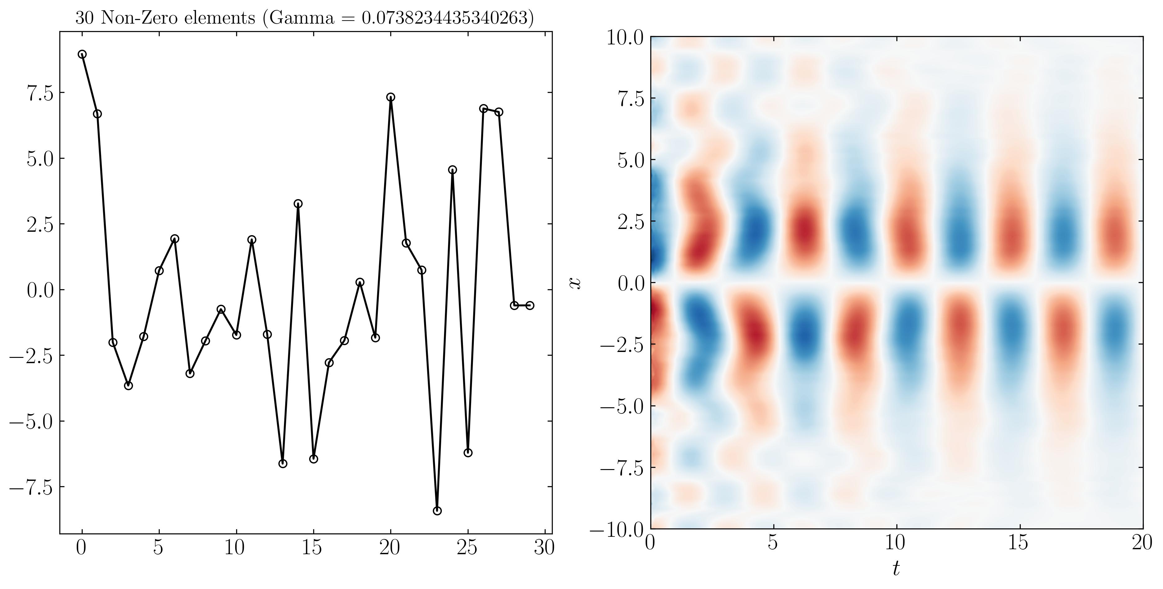
Here, Nz represents the number of non-zero modes in the solution, while PLoss indicates the performance loss — a normalized metric reflecting the overall model error resulting from using the optimal b. The attribute xpol contains the values of the optimal b corresponding to specific gamma values.
For instance, when $\gamma = 0.073$, we obtain 30 non-zero elements in the optimal b vector. Using this optimal b for reconstructing the DMD reduced model, we get the following result:
Similarly, we can reconstruct the system dynamics using only the 9, 3, and 2 most important DMD modes, as shown below:
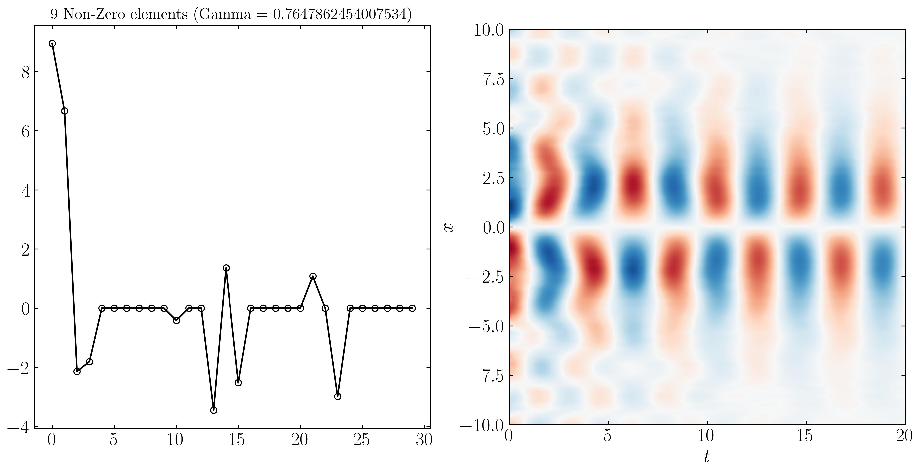
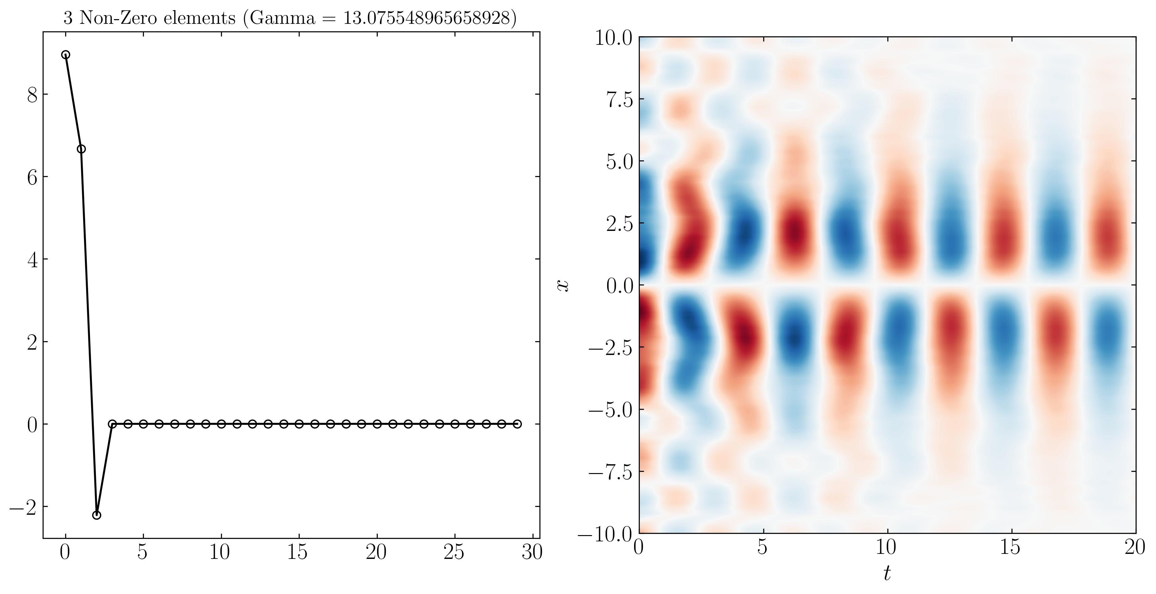
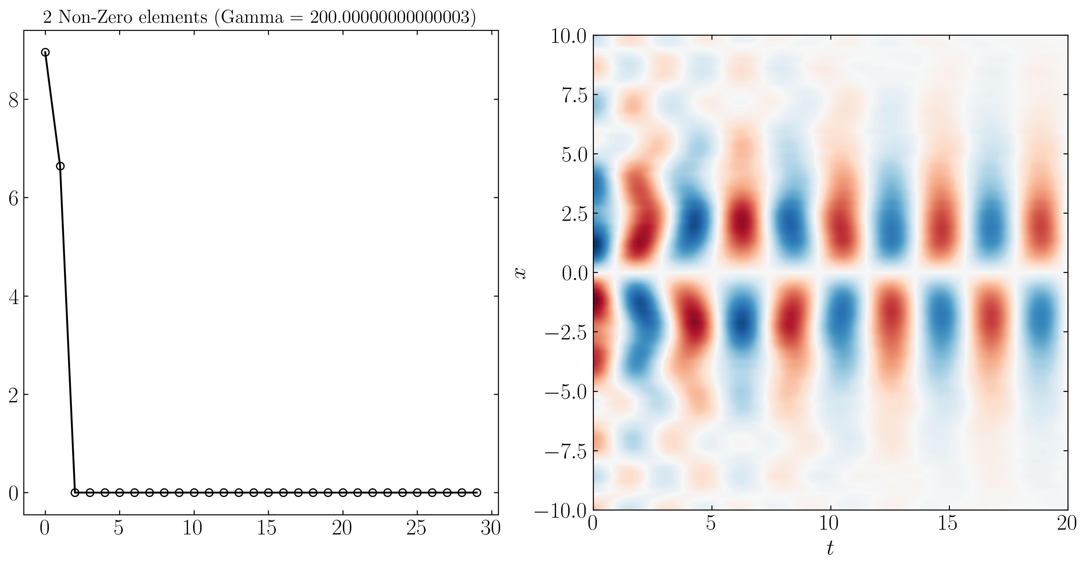
At higher resolutions, the first three modes are more distinguishable due to varying noise levels. Finally, SPDMD allows for a reconstruction using just a single mode — the most dominant mode that effectively captures the overall dynamics of the system. The power of SPDMD lies in its ability to selectively retain the most dominant modes while promoting sparsity. This approach ensures that the reconstructed model remains compact yet representative of the essential dynamics of the system.
Enjoy Reading This Article?
Here are some more articles you might like to read next: