In the world of data-driven modeling and signal processing, compressed sensing has emerged as a powerful technique for recovering signals from limited data. At the heart of this method lie two fundamental mathematical tools: the L1 and L2 norms. While they may seem abstract, their roles in promoting sparsity and ensuring stability are crucial for the success of compressed sensing algorithms. In this article, we will explore the significance of these norms, their differences, and how they contribute to efficiently reconstructing complex signals with minimal information.

The L1 and L2 norms are mathematical tools used to measure the size or magnitude of vectors, which are crucial for many optimization problems, including compressed sensing. They differ in how they calculate the magnitude of the vector, leading to different applications and characteristics. In this article, lets break down the mathematics behind L1 and L2 norms, understand how they are used in compressed sensing, and explore why the choice between them has profound implications for the accuracy and stability of the reconstructed signal.

Lets begin!!

L2 Norm

The most recognized of all norms is the L2 norm, also known as the Euclidean norm. The L2 norm is the square root of the sum of the squared values of the vector components—essentially, the root-mean-square of a given vector. Mathematically, it is represented as:

The L2 norm is straightforward, easy to implement, and has a natural, intuitive appeal. This simplicity is why it is widely used across many fields for measuring distances, regularization, and optimization. By minimizing the overall magnitude or energy, the L2 norm promotes smoothness, making it a critical tool for regularization and stability in various algorithms. One of the most notable applications of the L2 norm is in optimization, particularly through the least squares method. In linear regression and other optimization tasks, it minimizes the L2 norm of the difference between observed and predicted values, leading to optimal solutions. In physics, especially in classical mechanics, the L2 norm is used to quantify the kinetic energy of a system.

However, the L2 norm is not always the best choice, especially in machine learning. One key limitation is that it does not promote sparsity. When you minimize the L2 norm, it distributes non-zero values more evenly across all components, rather than driving many of them to zero. This can be problematic in applications like compressed sensing, where the goal is to recover a signal with only a few non-zero components.

Additionally, the L2 norm is sensitive to outliers because it squares each component’s value, which disproportionately emphasizes larger values. This sensitivity can skew results when the data contains outliers or significant errors, making it less robust in certain scenarios.

L1 Norm

L1 norm, also called the Manhattan norm or Taxicab norm, is the sum of the absolute values of the vector components. Mathematically, the L1 norm is defined as :

In the case of the L1 norm, instead of squaring each element as in the L2 norm, we simply take the absolute value. While this introduces challenges—such as discontinuities in its derivatives—the L1 norm has unique properties that make it particularly useful in specific applications. Compressed sensing leverages these properties to great effect.

A key advantage of the L1 norm is its ability to promote sparsity. It encourages solutions where many components of the vector are zero or near zero. This is crucial for compressed sensing, as it enables the reconstruction of signals from a limited number of measurements by focusing on only the most significant components. Thanks to this sparsity, the L1 norm is ideal for recovering signals in fields like medical imaging (e.g., MRI) and data compression, where efficiency and accuracy are paramount, even with incomplete data.

Norms at play

Now lets visualize the difference between L1 and L2 Norms. For this, we’ll start by generating a random linear dataset based on the following expression :

where 𝛿 represents normally distributed noise with a standard deviation of 0.5, which will introduce several outliers into the dataset.

Using this dataset, we’ll fit two lines—one using the L1 norm criterion and the other using the L2 norm criterion—highlighting how each norm handles the data differently, particularly in the presence of outliers.

To begin, load the necessary Python modules in a Jupyter notebook:

import matplotlib.pyplot as plt
import numpy as np
import pandas as pd
import fluidfoam as fl
import scipy as sp
import scipy.optimize as spopt
import scipy.fftpack as spfft
import scipy.ndimage as spimg
import cvxpy as cvx
%matplotlib inline
plt.rcParams.update({'font.size' : 14, 'font.family' : 'Times New Roman', "text.usetex": True})

# Path to save files
savePath = 'E:/Blog_Posts/OpenFOAM/ROM_Series/Post37/'

Now, let’s generate the dataset:

x = np.sort(np.random.uniform(-10, 10, 20))
y = 0.4 * x + 3 + 0.5 * np.random.randn(len(x))

Next, using the SciPy optimize package, we’ll fit lines to the dataset using both the L1 and L2 norms:

# L1 fitting function
l1_fit = lambda x0, x, y: np.sum(np.abs(x0[0] * x + x0[1] - y))
xopt1 = spopt.fmin(func=l1_fit, x0=[1, 1], args=(x, y))

# L2 fitting function
l2_fit = lambda x0, x, y: np.sum(np.power(x0[0] * x + x0[1] - y, 2))
xopt2 = spopt.fmin(func=l2_fit, x0=[1, 1], args=(x, y))

Finally, let’s visualize the dataset and the fit lines:

fig, ax = plt.subplots()

ax.plot(x, y, 'o', label='Data')
ax.plot(x, xopt1[0] * x + xopt1[1], color='k', ls='--', label=r'$L_1$' + ' fit')
ax.plot(x, xopt2[0] * x + xopt2[1], color='k', ls='-', label=r'$L_2$' + ' fit')

ax.set_xlabel(r'$x$')
ax.set_ylabel(r'$y$')

ax.xaxis.set_tick_params(direction='in', which='both')
ax.yaxis.set_tick_params(direction='in', which='both')
ax.xaxis.set_ticks_position('both')
ax.yaxis.set_ticks_position('both')

ax.legend(loc='best', frameon=False)

plt.show()

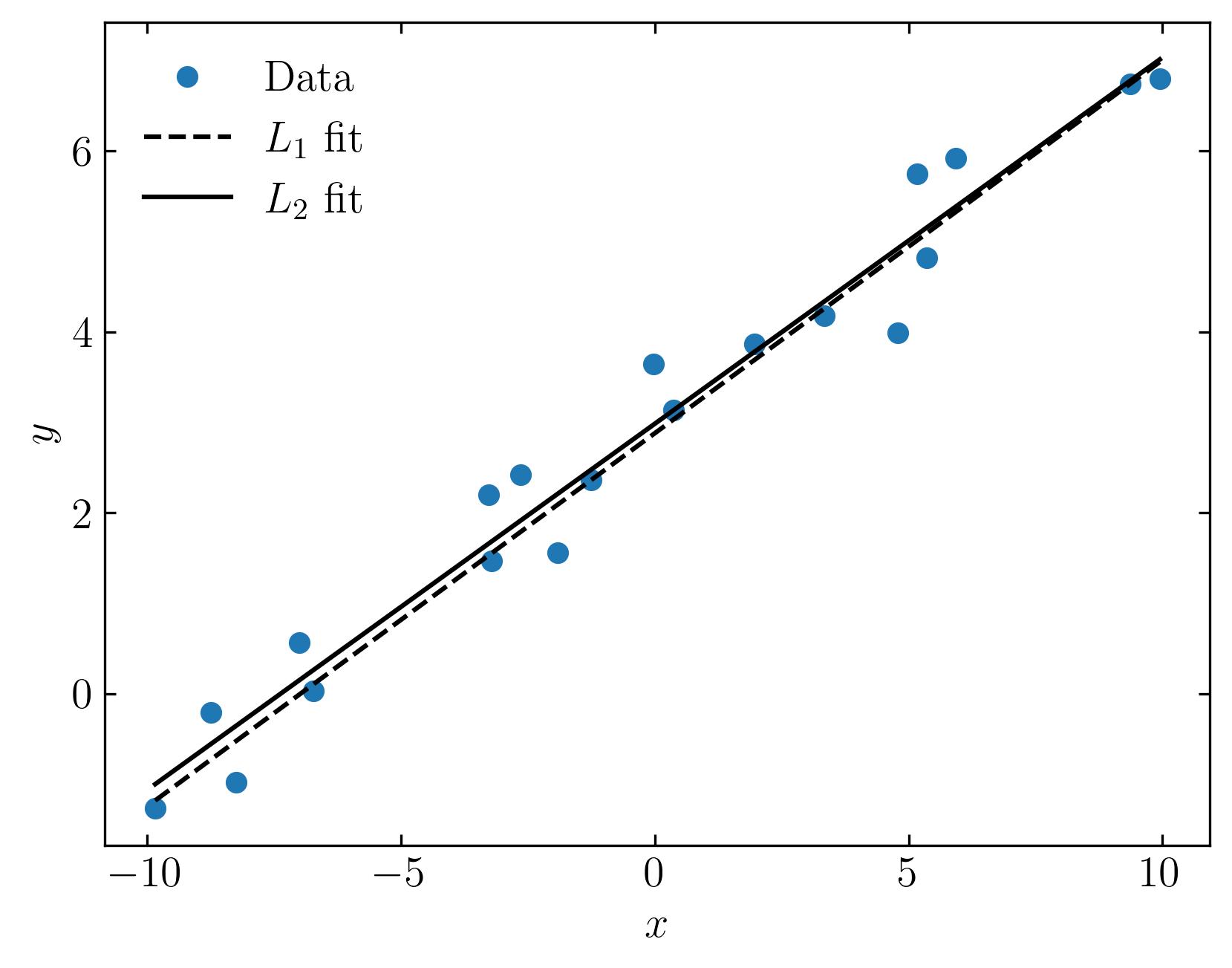
Both lines fit the data reasonably well, despite the presence of some noise due to the normally distributed error. While neither fit is perfect, the influence of outliers on the L2 norm is more pronounced.

Now, let’s introduce more outliers to see how the fits respond. We’ll perturb a couple of data points by shifting them far from the lines. This simulates a common real-world scenario where outliers occur, creating challenges for fitting models:

# generate some Outliers
y2 = y.copy()
y2[1] += 8
y2[17] -= 6

# Refit the data
xopt12 = spopt.fmin(func=l1_fit, x0=[1, 1], args=(x, y2))
xopt22 = spopt.fmin(func=l2_fit, x0=[1, 1], args=(x, y2))

# Replot the data

fig, ax = plt.subplots()
ax.plot(x, y2, 'o', label='Data')
ax.plot(x, xopt12[0] * x + xopt12[1], color='k', ls='--', label=r'$L_1$' + ' fit')
ax.plot(x, xopt22[0] * x + xopt22[1], color='k', ls='-', label=r'$L_2$' + ' fit')
ax.set_xlabel(r'$x$')
ax.set_ylabel(r'$y$')
ax.xaxis.set_tick_params(direction='in', which='both')
ax.yaxis.set_tick_params(direction='in', which='both')
ax.xaxis.set_ticks_position('both')
ax.yaxis.set_ticks_position('both')
ax.legend(loc='best', frameon=False)
plt.show()

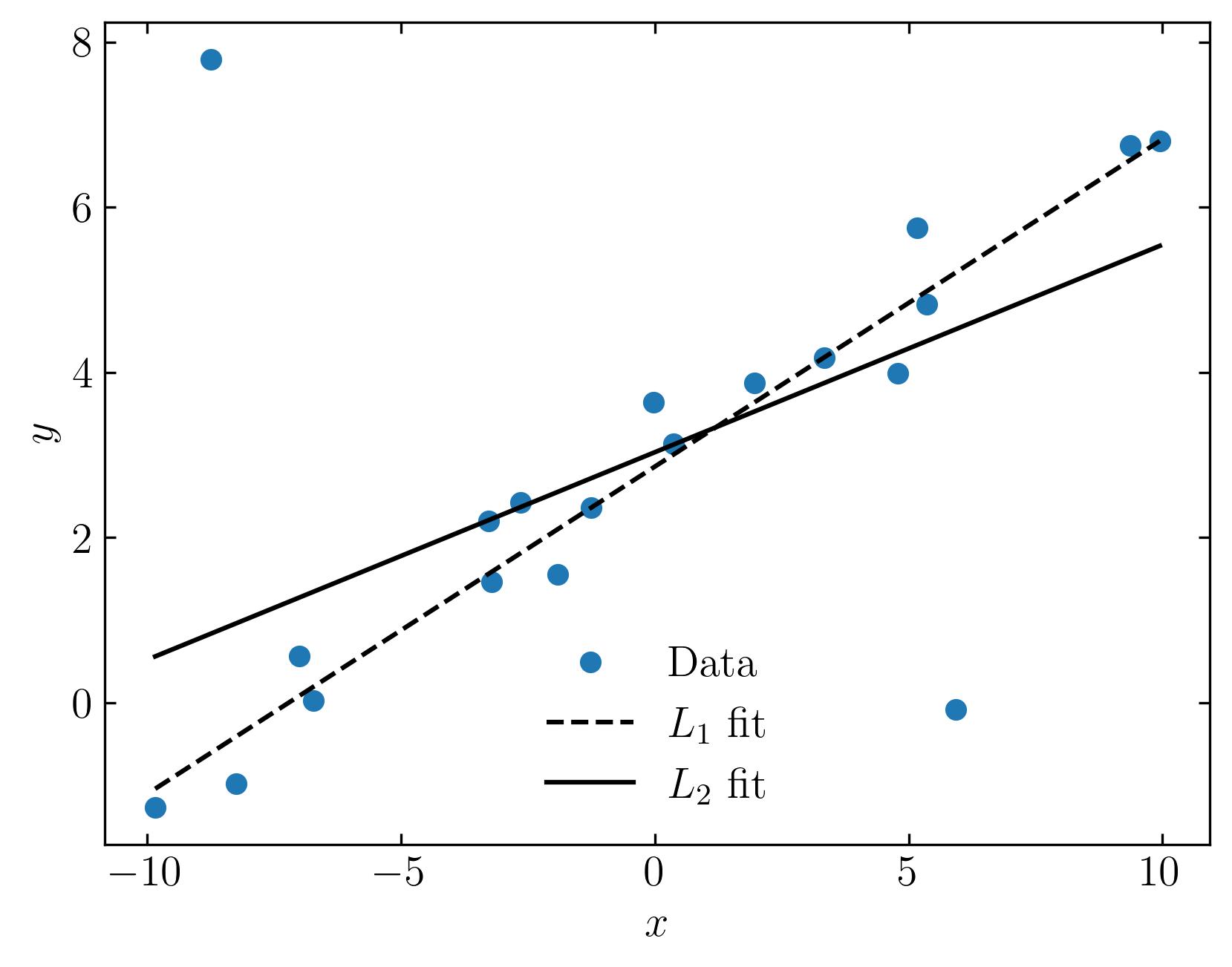
As you can see, the results are quite revealing. The L1 fit stays true to the general trend of the data, while the L2 fit is skewed by the outliers.

This brings us to a key distinction: In the L2 norm, errors are squared, meaning outliers have a disproportionately large impact. On the other hand, the L1 norm treats outliers more gently by considering only their absolute values. This results in a cleaner, more robust fit that aligns better with our intuition of what a good fit should look like, especially in the presence of outliers.

In conclusion, both the L1 and L2 norms have their strengths and limitations, and understanding their distinct roles is key to choosing the right tool for different tasks. The L2 norm is ideal for applications where smoothness and stability are critical, but its sensitivity to outliers can be a drawback in noisy datasets. On the other hand, the L1 norm shines in situations where robustness to outliers and sparsity are essential, such as compressed sensing and data recovery. Ultimately, the choice between L1 and L2 norms depends on the nature of your data and the specific goals of your model. By leveraging the unique advantages of each, you can build more effective solutions across a wide range of applications. In the next blog, lets explore one such application of these norms - compressed sensing!