In the world of data acquisition, the need for high-resolution measurements often comes with a cost—both in terms of time and resources. Compressed sensing offers a paradigm shift by allowing us to reconstruct high-fidelity signals from a small number of measurements, challenging traditional sampling techniques. This article explores the core principles of compressed sensing and demonstrates how sparse representations can be leveraged to recover information efficiently, making it a powerful tool in fields ranging from medical imaging to signal processing.

Compressed sensing (CS) is a signal processing technique that enables the reconstruction of sparse or compressible signals using fewer measurements than traditional methods typically require. It leverages the idea that many natural signals or datasets possess inherent sparsity — meaning they can be represented by a relatively small number of significant components in a suitable basis, such as Fourier or wavelet transforms.

The fundamental assumption in compressed sensing is that a signal is sparse in a particular domain. While the signal may appear complex or dense in its original form, it can often be expressed using only a few significant components (or coefficients) when transformed into a different basis. For instance, a signal that seems intricate in the time domain may have only a handful of dominant frequency components in the Fourier domain. This is akin to how power spectral density is interpreted in fluid dynamics. Another example is image compression, where natural images can be approximated with only a few wavelet coefficients.

Traditional signal processing follows the Nyquist-Shannon sampling theorem, which requires sampling a signal at twice its highest frequency to fully reconstruct it. In contrast, compressed sensing enables undersampling—collecting fewer measurements than the Nyquist rate suggests—while still achieving accurate signal reconstruction. This is made possible through the concept of incoherence, where the signal’s sparsity in one domain (e.g., frequency) is incoherent with the way measurements are taken in another domain (e.g., time). This allows for the recovery of the original signal, even with a reduced number of measurements.

Compressed sensing involves two critical steps. First, during data measurement, the signal is sampled indirectly through a set of random or linear measurements, rather than through direct sampling. The second step is reconstruction, where an optimization process is applied to recover the original signal. The most common approach is solving a convex optimization problem, such as L1-norm minimization or basis pursuit, which seeks the sparsest signal that fits the available measurements.

Mathematics Behind Compressed Sensing

Given a signal $x~\epsilon~\mathbb{R^n}$, we can assume that it has a sparse representation (is K-Sparse) in a basis $\Psi~\epsilon~\mathbb{R^{n\times n}}$ such that :

where 𝛼 is a K-sparse vector, meaning it contains exactly K non-zero elements.

If the signal x is K-sparse in $\Psi$, we can collect a sub-sample of measurements $y~\epsilon~\mathbb{R^m}$, where $m\ll n$, instead of measuring x directly and then compressing it. These measurements are gathered using a sensing matrix $\Phi~\epsilon~\mathbb{R^{m\times n}}$, such that:

These sub-sampled measurements can be random projections of the original signal x, where the entries of Φ are Gaussian-distributed random variables. Alternatively, individual entries of x, such as single pixels in the case of an image, may be measured directly, where the rows of Φ contain zeros except for a single unit entry per row.

The challenge in compressed sensing is recovering x from y, even when 𝑚 is much smaller than 𝑛. If we know the sparse vector 𝛼, we can reconstruct the full signal x using:

Since this system is underdetermined (more unknowns than equations), there could be infinitely many solutions for 𝛼. The goal is to find the sparsest solution 𝛼 that satisfies the following optimization problem:

$\alpha = \min(\vert\vert\alpha\vert\vert _0)$ such that $y = \Phi \Psi \alpha$

Here, ∣∣α∣∣0 represents the number of non-zero elements in 𝛼. Unfortunately, this is a non-convex optimization problem, which can only be solved by an exhaustive brute-force search. The computational complexity of such a search grows combinatorially with n and K, making it an NP-hard problem. This makes solving even moderately large problems infeasible with current computational power.

However, we can relax the problem to a convex optimization by minimizing the L1 norm:

$\alpha = \min(\vert\vert\alpha\vert\vert _1)$ such that $y = \Phi \Psi \alpha$

L1 norm minimization encourages sparsity in the solution. Under this formulation, the optimization almost always leads to a sparse solution, provided the measurements in Φ are incoherent with respect to the basis Ψ, meaning the two are uncorrelated.

Compressed Sensing In Fluid Dynamics

Compressed sensing has wide-ranging applications. For instance, consider medical imaging. In MRI (magnetic resonance imaging), compressed sensing is used to reduce the time needed to collect data, while still producing high-quality images from fewer measurements. In astronomy, compressed sensing is applied to recover high-resolution images of astronomical objects from limited data. In communications and data storage, it helps to reduce the amount of data required to be transmitted or stored while retaining essential information. And finally in Fluid Dynamics, compressed sensing is used for sparse data reconstruction, sensor placement, and modal decomposition.

Lets focus on a few key advantages of Compressed sensing from the description of application above. Compressed sensing firstly allows data collection from fewer measurements, leading to faster and more cost-effective data acquisition. Second, it reduces storage requirements by storing only the most important components. And most importantly, Compressed sensing methods are often robust to noise, allowing accurate recovery even with imperfect measurements. All these advantages are seen in action in Fluid dynamics. It leverages the fact that many fluid dynamics phenomena exhibit sparse representations in certain bases, such as wavelets, Fourier, or proper orthogonal decomposition (POD) modes. Thus, in fluid dynamics, compressed sensing is applied in context of sparse data reconstruction and modal decomposition techniques.

Lets look at a few examples in detail :

1. Sparse Data Reconstruction : In experimental fluid dynamics, obtaining high-resolution data can be expensive or difficult (e.g., in particle image velocimetry or pressure measurements). Compressed sensing allows for the reconstruction of flow fields from a limited number of measurements by exploiting sparsity in some transform domain. For instance, fewer sensor points can be used to reconstruct full velocity fields, reducing data collection time and cost. In another example, limited pressure measurements can be reconstructed to obtain full-field pressure data in turbulent flows using compressed sensing techniques.
2. Modal Decomposition : Compressed sensing has been used in conjunction with modal decomposition methods like Dynamic Mode Decomposition (DMD) and Proper Orthogonal Decomposition (POD). These methods represent complex flow fields with a few dominant modes, making the data inherently sparse in the modal domain. For example, compressed sensing principles are used with Dynamic Mode Decomposition (DMD) in a variant names Sparsity-Promoting DMD (SPDMD).
3. Reduced Order Models (ROMs) : Compressed sensing helps in building efficient ROMs by identifying key modes from sparse or under-sampled data, making the computational cost lower while retaining accuracy.
4. Flow Reconstruction in Time-Resolved Data : When dealing with time-resolved fluid dynamics data (e.g., turbulent wake behind a bluff body), the spatial and temporal data can be sparse, and compressed sensing helps recover complete data from few-time snapshots or low-resolution measurements.

Compressed Sensing in Action

Let’s consider a simple example to demonstrate compressed sensing in action. In this case, we will generate an artificial signal—think of it as a sound wave or a sensor signal from PIV measurements—and attempt to reconstruct the original signal using only about 3% of the data. This example will showcase one-dimensional, temporal compressed sensing.

First, let’s load the necessary modules in a Jupyter notebook:

import matplotlib.pyplot as plt
import numpy as np
import pandas as pd
import fluidfoam as fl
import scipy as sp
import scipy.optimize as spopt
import scipy.fftpack as spfft
import scipy.ndimage as spimg
import cvxpy as cvx
%matplotlib inline
plt.rcParams.update({'font.size' : 14, 'font.family' : 'Times New Roman', "text.usetex": True})

# Path to save files
savePath = 'E:/Blog_Posts/OpenFOAM/ROM_Series/Post38/'

The signal we will consider, taken from the book “Dynamic Mode Decomposition: Data-Driven Modeling of Complex Systems” by J. Nathan Kutz and others, is a two-tone signal in time:

To accurately resolve the high-frequency component of 531 Hz, the Nyquist sampling theorem dictates that the signal must be sampled at least twice its highest frequency, which would require 1062 samples per second. For simplicity, we’ll oversample by a factor of four, collecting 4096 samples over a one-second interval.

Let’s generate the signal:

n = 4096 # number of samples
p = 128 # number of sub-samples 
t = np.linspace(0, 1, n) 
y = np.sin(73 * 2* np.pi * t) + np.sin(531 * 2 * np.pi * t)     
yt = spfft.dct(y, norm='ortho')
psd = np.abs(yt) ** 2
frequency = np.linspace(0, 1, n) * (n // 2)

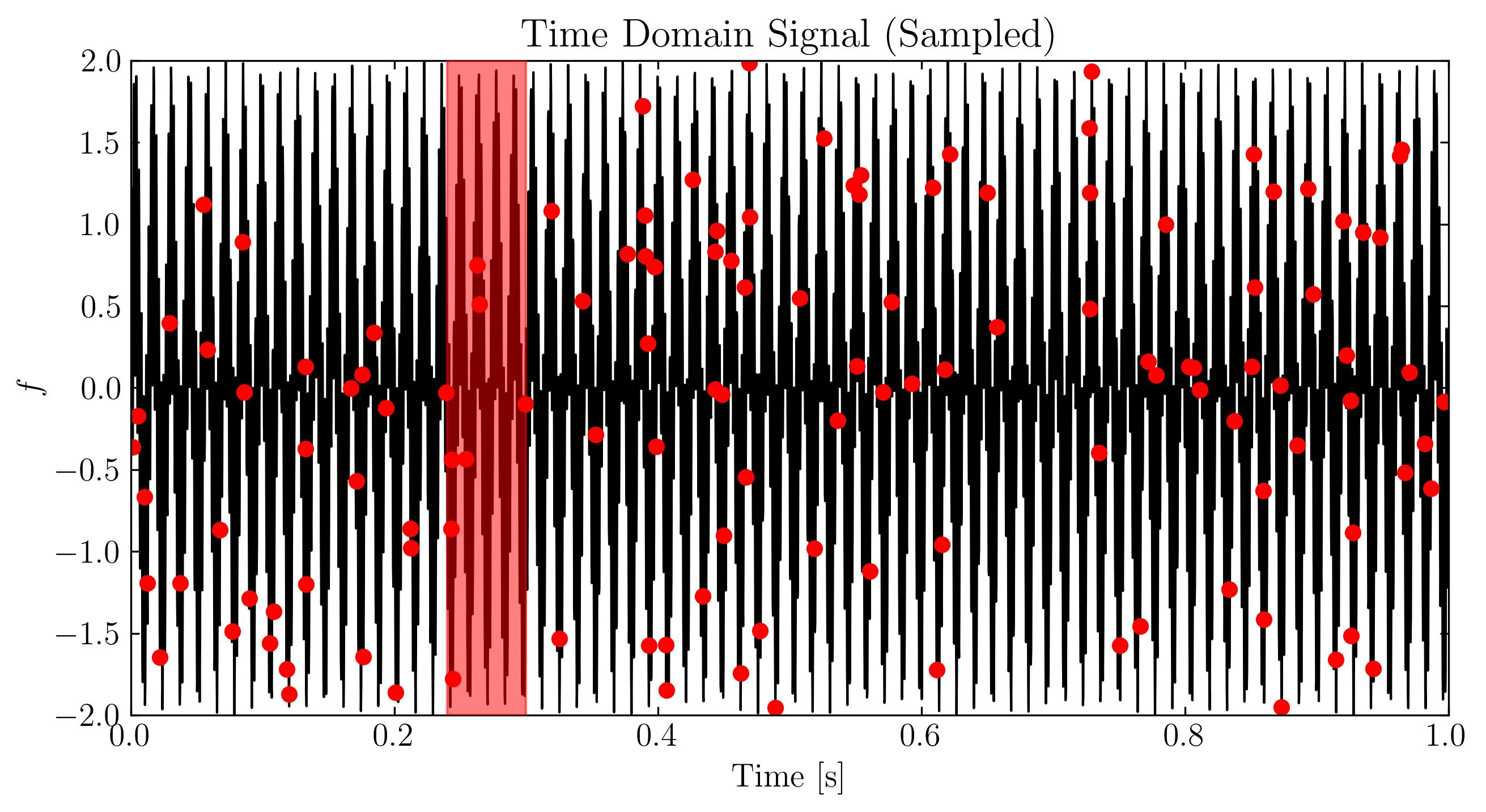
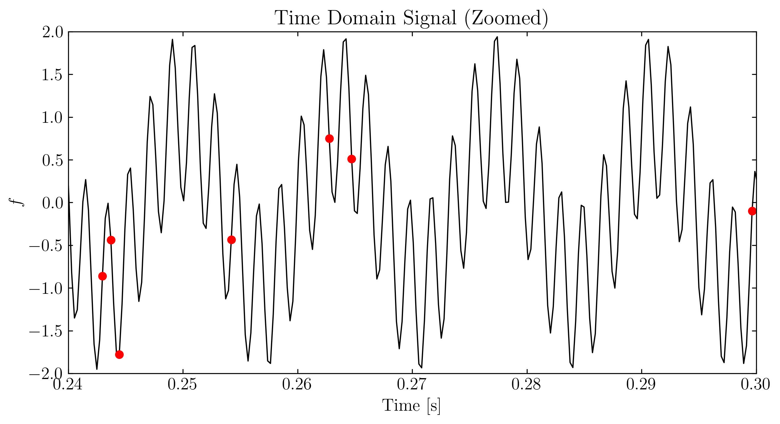
Next, we can visualize these signals using standard matplotlib routines. Below, I will display the signal in three forms: the original time-domain signal, a zoomed-in section of the time-domain signal, and the signal in the frequency domain.

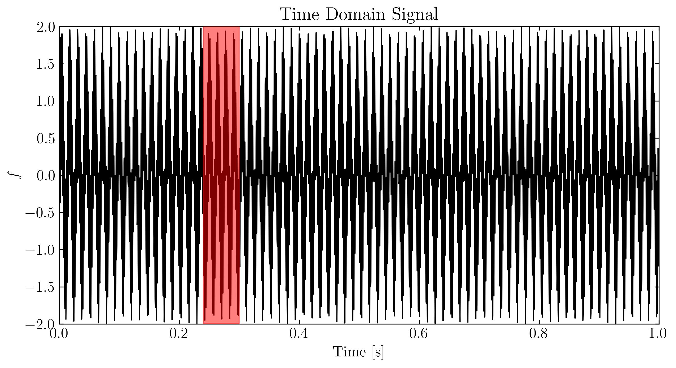
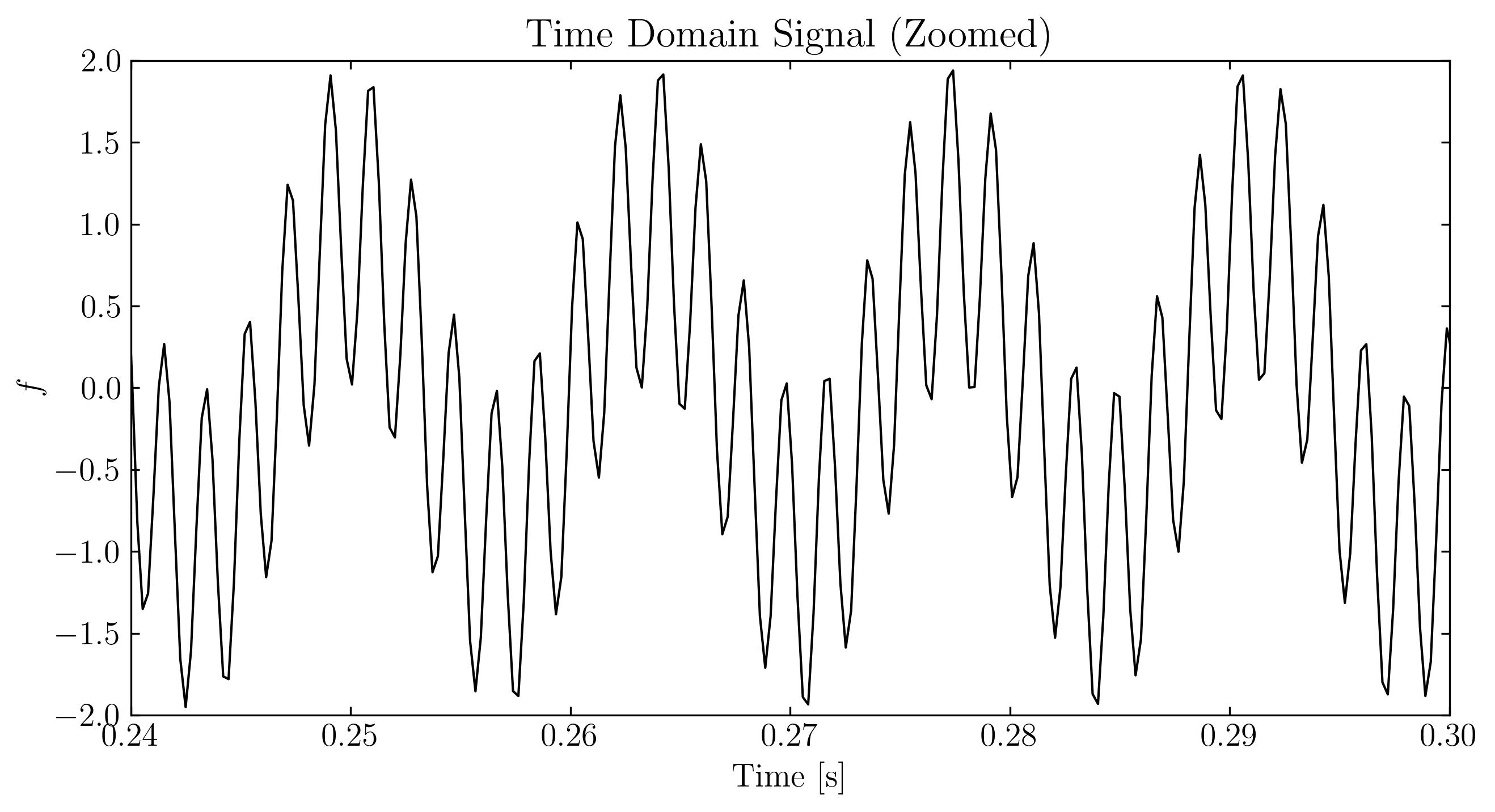
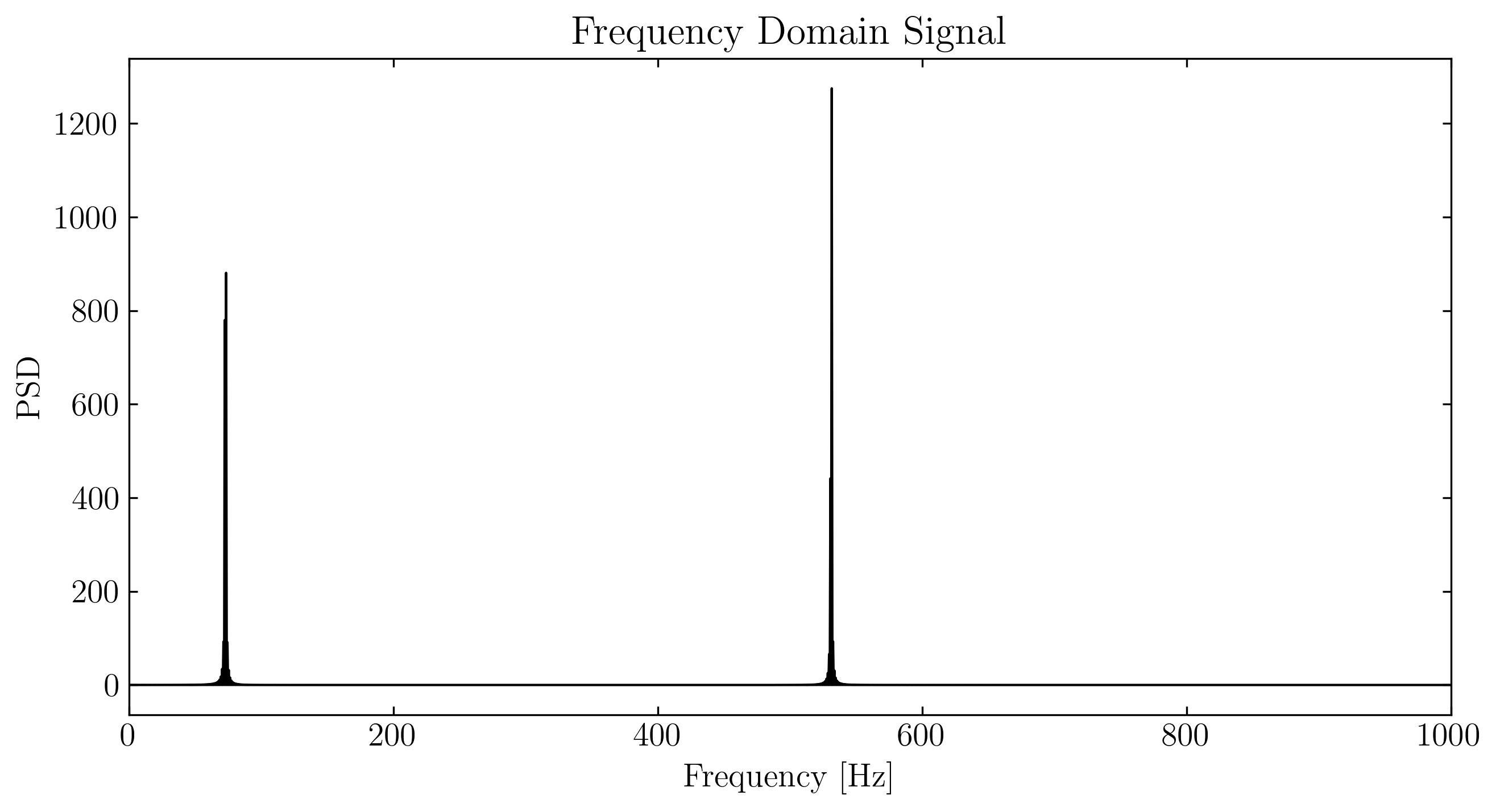
As we can see, the signal exhibits a clear and non-trivial pattern. Additionally, this signal is extremely sparse in the Fourier (frequency) domain, with only two non-zero frequency components—73 Hz and 531 Hz. Now, let’s sample approximately 3% of the temporal signal. For simplicity, we will sample at a rate of 128 samples per second, which is 1/8 of the Nyquist rate. This gives us the compressed measurement:

where Φ is derived using the inverse discrete cosine transform (iDCT).

Let’s visualize the sampled signal:

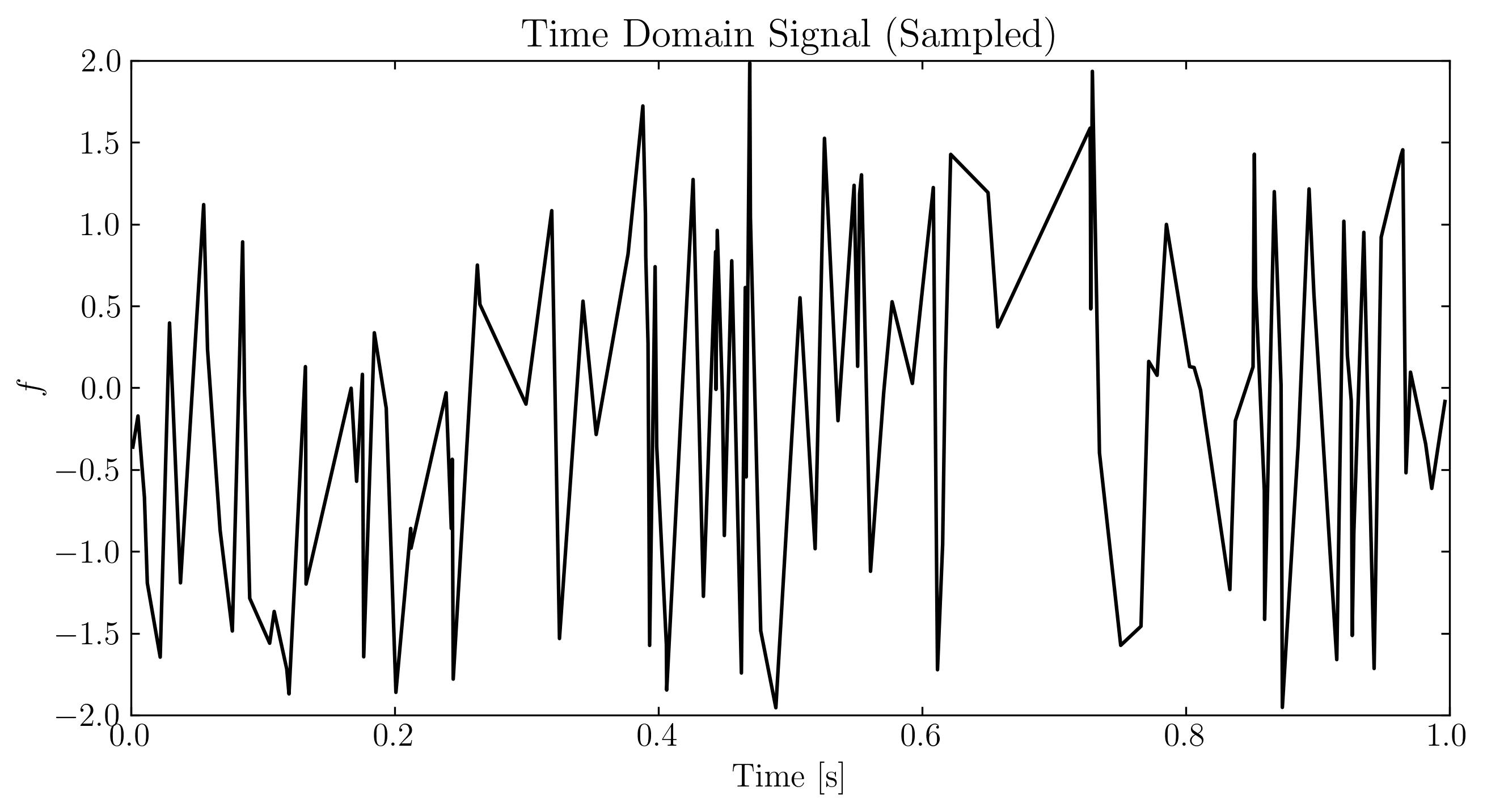
At first glance, this sampled signal might seem like noise. However, the underlying signal—and its frequency content—remains unchanged. The challenge now is to extract the two dominant frequencies from this incomplete data and attempt to reconstruct the original signal. This is where compressed sensing comes into play.

In this context, compressed sensing works because the signal’s frequency content is highly sparse. This is where the L1 norm minimization comes in. Out of all possible signals, we aim to find the simplest one that aligns with the known data. Specifically, we want to find a set of frequencies that satisfy two conditions: (a) the reconstructed signal matches the available data as closely as possible, and (b) the L1 norm of the frequencies is minimized. This approach will yield a sparse solution—exactly what we’re looking for. In Python, we will use the convex optimization library (CVXPY) to minimize the norm and reconstruct the signal.

To perform the minimization, we will frame our problem as a linear system of equations, 𝐴𝑋=𝐵. Our goal is to derive a matrix 𝐴 that, when multiplied with a candidate solution X, yields B, the vector of sampled data. In this case, X exists in the frequency domain, while B is in the temporal domain. The matrix A performs both sampling and transformation from spectral to temporal domains, which is key to compressed sensing.

Let’s assume 𝐹 is the target signal and 𝜙 is the sampling matrix. Then, 𝐵=𝜙𝐹. Next, let 𝜓 be a matrix that transforms the signal from the frequency domain to the time domain using the inverse discrete cosine transform (iDCT). Given a solution 𝑋 in the frequency domain, this transformation is performed using 𝜓𝑋=𝐹. Putting it all together, we arrive at the linear system 𝐴𝑋=𝐵, where 𝐴=𝜙𝜓. The matrix 𝜓 is straightforward to construct—it’s the iDCT applied to the columns of the identity matrix, and 𝜓𝑋 is equivalent to applying the iDCT to 𝑋.

Let’s now perform this minimization:

# iDCT matrix A
A = spfft.idct(np.identity(n), norm='ortho', axis=0)
A = A[ri]

# L1 minimization
vx = cvx.Variable(n)
objective = cvx.Minimize(cvx.norm(vx, 1))
constraints = [A*vx == y2]
prob = cvx.Problem(objective, constraints)
result = prob.solve(verbose=True)

Now that we’ve constructed the A matrix and run the minimization, we can reconstruct the signal by transforming the solution from the frequency domain back to the time domain.

# Reconstruct the signal
x = np.array(vx.value)
x = np.squeeze(x)
sig = spfft.idct(x, norm='ortho', axis=0)
PSD = np.abs(spfft.dct(sig, norm='ortho')) ** 2
Frequency2 = np.linspace(0, 1, n) * (n // 2)

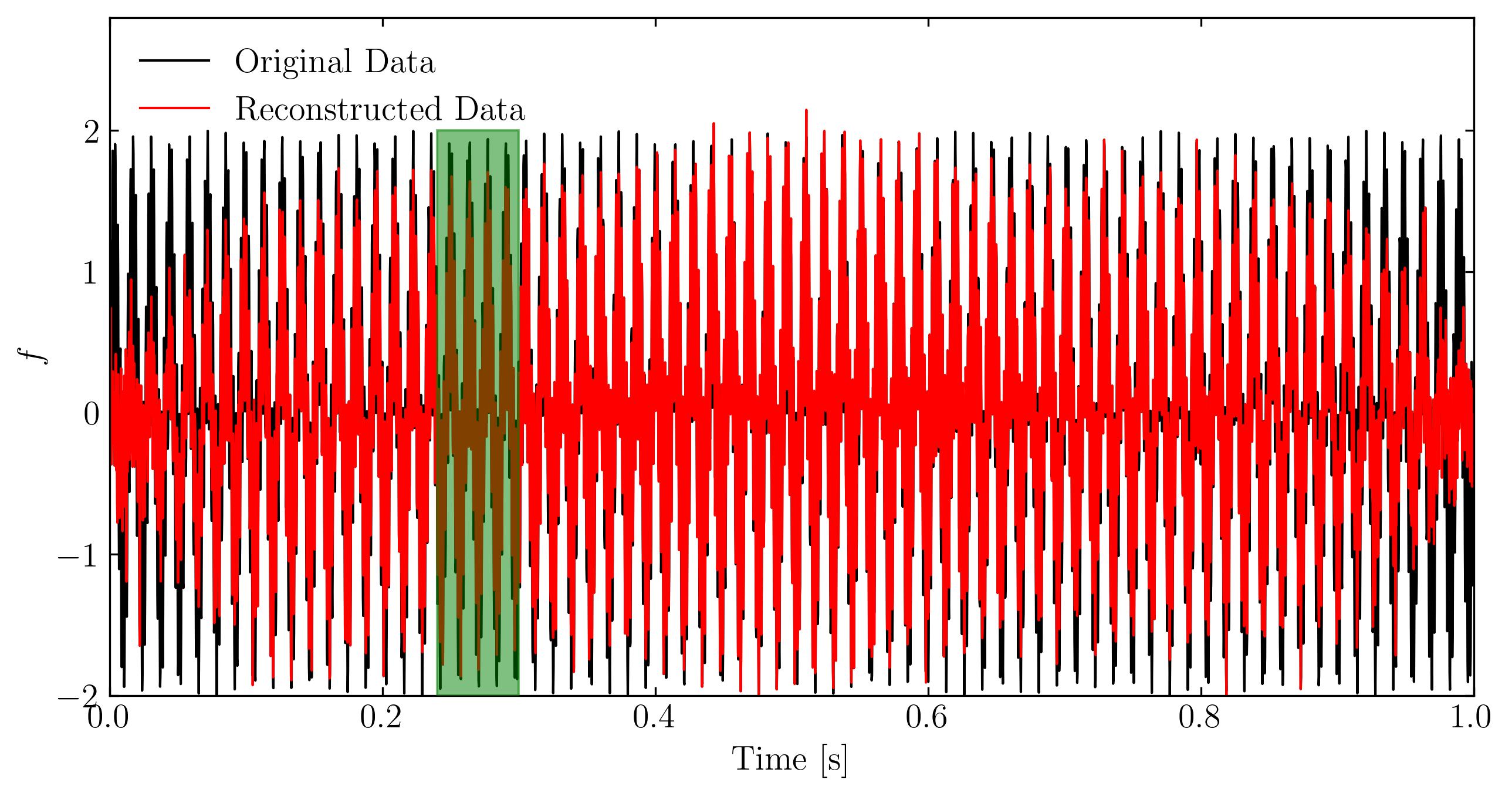
Now, let’s visualize the signals again, but this time we’ll compare the reconstructed signal with the original one.

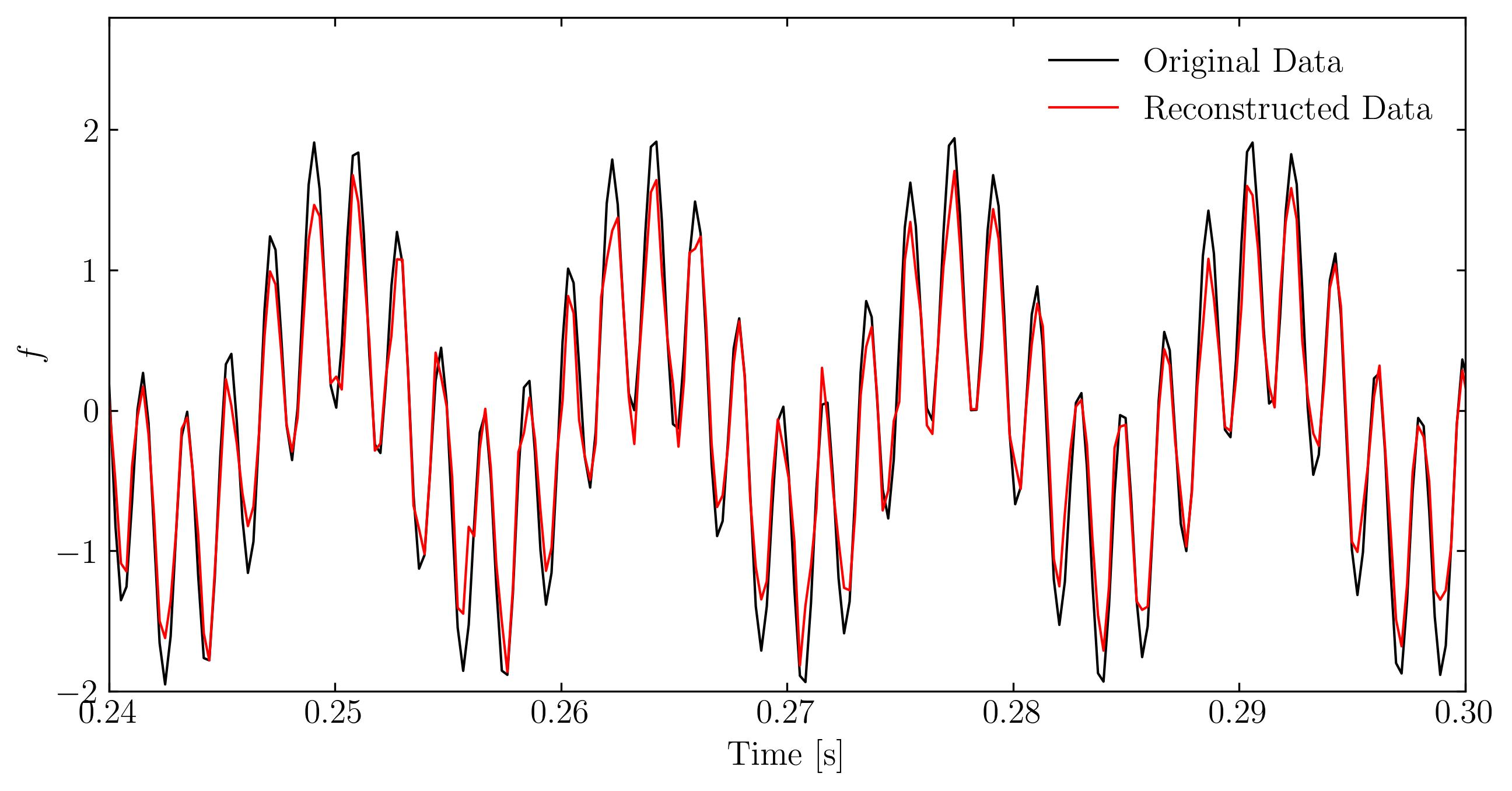
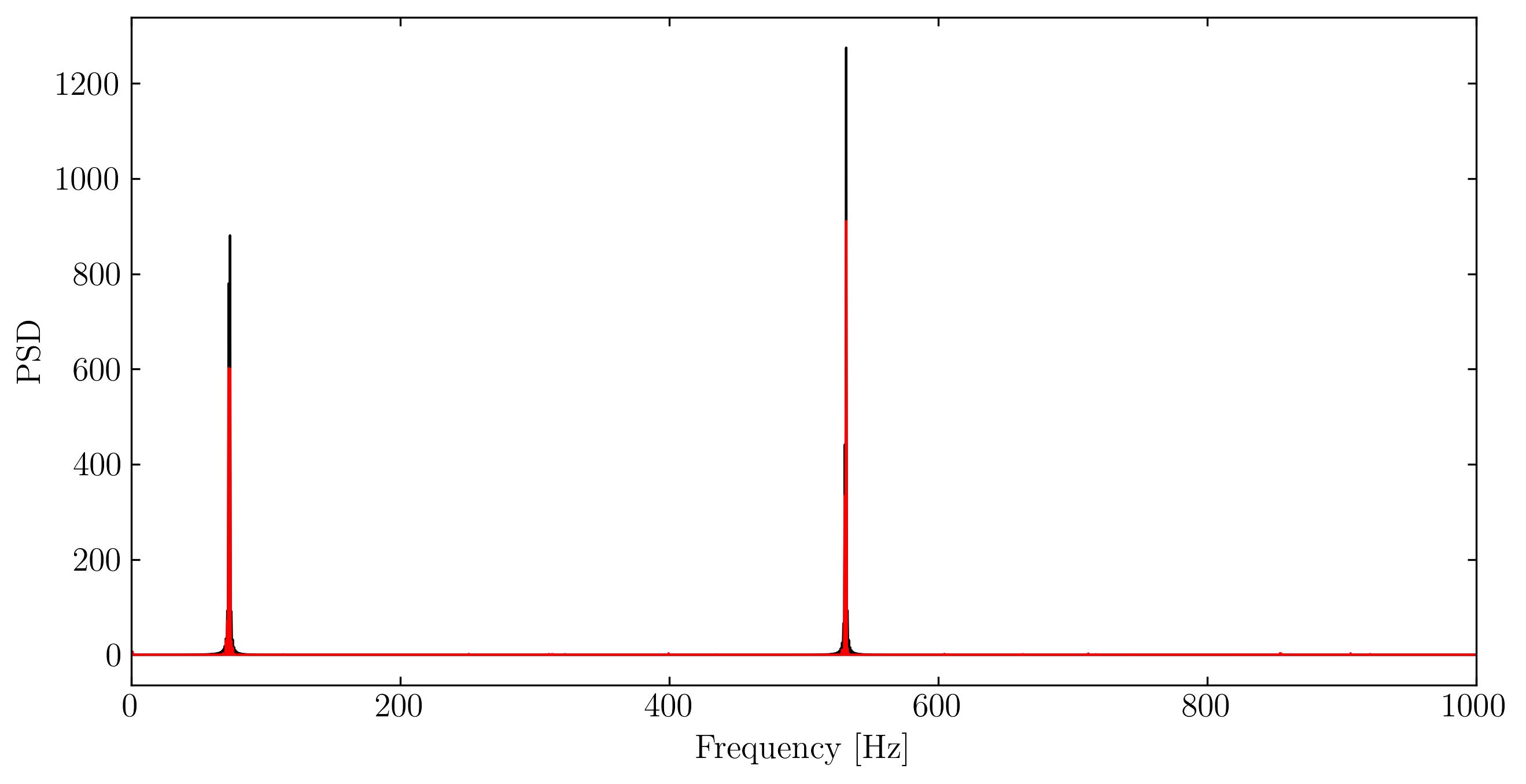
From the zoomed-in figure and the overall frequency trends, we can see that the reconstruction is quite accurate, especially considering that we used only 3% of the sub-sampled data. However, one noticeable issue is the degradation of the reconstruction quality around t=0 and t=1. This is likely due to the sample interval violating the periodic boundary conditions required by the cosine transform. Without prior knowledge of the signal’s nature, it’s difficult to avoid such violations in an arbitrary signal sample.

The good news is that we now have clear indications of the true frequencies of the original signal. If needed, we could go back and resample the signal within an interval that satisfies periodic boundary conditions for better accuracy.