Revealing Complex Dynamics with Multi-Resolution Dynamic Mode Decomposition

17 minute read

Published: November 11, 2024

Data-driven analysis has unlocked new ways to decipher complex systems, with Dynamic Mode Decomposition (DMD) becoming a cornerstone method for identifying coherent structures in data. Yet, standard DMD techniques often fall short when it comes to capturing the multi-scale characteristics common in dynamic phenomena. This is where Multi-Resolution Dynamic Mode Decomposition (MRDMD) comes in. MRDMD is a powerful extension that deconstructs data across multiple scales, revealing patterns that are otherwise hidden. In this article, lets explore how MRDMD enhances our ability to analyze complex datasets, its unique methodology, and the insights it brings to data-driven modeling.

Dynamic Mode Decomposition (DMD) has emerged as a powerful tool in data-driven analysis, especially for identifying coherent structures within complex datasets. However, despite its capabilities, DMD comes with some key limitations. One major challenge is its difficulty in capturing multi-scale dynamics, as well as its reliance on fixed temporal scales, which often leads to missing important transient features in the data. These issues were explored in my previous articles, where we saw how DMD’s lack of adaptability impacts its performance when applied to systems that exhibit variations across different scales.

To address these shortcomings, Multi-Resolution Dynamic Mode Decomposition (MRDMD) provides a promising solution. By breaking down data across multiple temporal resolutions, MRDMD captures a more detailed and nuanced view of dynamic systems, uncovering patterns that traditional DMD may overlook. MRDMD is a versatile and powerful technique for extracting dynamic structures from time-series datasets. Its strength lies in its ability to identify features at varying time scales. This is achieved by recursively parsing through the data and performing DMD on sub-sampled datasets. The result is a richer analysis that reveals the underlying dynamics at both temporal and spatial scales.

Let’s dive in and explore MRDMD in more detail!

Multi-resolution dataset

Let’s start by constructing a toy dataset that contains multiple time scales, including a one-time event. Using this dataset, we will first attempt a standard DMD analysis, explore its limitations, and demonstrate why a multi-resolution method like MRDMD is necessary.

To begin, let’s open a Jupyter notebook and load the required modules:

import numpy as np
import matplotlib.pyplot as plt
from numpy import dot, multiply, diag, power
from numpy import pi, exp, sin, cos
from numpy.linalg import inv, eig, pinv, solve
from scipy.linalg import svd, svdvals
from math import floor, ceil 
%matplotlib inline
plt.rcParams.update({'font.size' : 14, 'font.family' : 'Times New Roman', "text.usetex": True})

# Path to save files
savePath = 'E:/Blog_Posts/OpenFOAM/ROM_Series/Post39/'

Let’s consider a toy dataset consisting of 80 locations or signals (along the x-axis), each sampled 1600 times at a constant rate over time (the t-axis).

# Define time and space domains
x = np.linspace(-12, 12, 80)      # Spatial range
t = np.linspace(0, 20, 1600)      # Time range
Xm, Tm = np.meshgrid(x, t)

# Create data with a variety of spatial and temporal features
D = np.exp(-np.power(Xm / 3, 2)) * np.exp(1.0j * Tm)             # Gaussian shape with oscillation in time
D += np.sin(1.0 * Xm) * np.exp(1.5j * Tm)                        # Sinusoidal spatial pattern with temporal oscillation
D += 0.8 * np.cos(1.2 * Xm) * np.exp(2.5j * Tm)                  # Additional spatial and temporal frequency
D += 0.5 * np.sin(1.4 * Xm) * np.exp(4.0j * Tm)                  # Higher temporal frequency and smaller amplitude
D += 0.5 * np.cos(1.6 * Xm) * np.exp(5.0j * Tm)                  # Higher frequency cosine term
D += 0.3 * np.sin(2.3 * Xm) * np.exp(7j * Tm)                    # Another high-frequency component with variation
D += 0.3 * np.cos(2.4 * Xm) * np.exp(9j * Tm)                    # Cosine term with increased temporal frequency
D += 0.15 * np.sin(6.0 * Xm) * np.exp(11j * Tm)                  # Smaller amplitude, faster oscillation
D += 0.15 * np.cos(6.2 * Xm) * np.exp(13j * Tm)                  # Matching cosine term for symmetry
D += 0.1 * np.random.randn(*Xm.shape)                            # Add noise for realism

# Add a Gaussian pulse that moves slowly over time for additional complexity
D += 3 * np.exp(-np.power((Xm + 6) / 4, 2)) * np.exp(-np.power((Tm - 10) / 4, 2))

# Add spatial and temporal blocks to introduce abrupt transitions and patterns
D[:600, 30:] += 1.5
D[400:800, 45:65] -= 2
D[1000:, :25] -= 1.5
D[1200:1400, 15:35] += 2.5
D[900:1100, 55:75] += 2
D[1300:1380, 55:75] += 2
D[1460:1540, 55:75] += 2
D = D.T  # Transpose for consistency with input-output extraction

# Extract input-output matrices
X = D[:, :-1]     # All columns except the last
Y = D[:, 1:]      # All columns except the first

Firstly, lets visualize this dataset:

fig, ax = plt.subplots()
p = ax.contourf(x, t, D.T, levels = 501, cmap = 'RdBu')
ax.xaxis.set_tick_params(direction='in', which='both')
ax.yaxis.set_tick_params(direction='in', which='both')
ax.xaxis.set_ticks_position('both')
ax.yaxis.set_ticks_position('both')
ax.set_aspect('equal')
ax.set_xlabel(r'$x$')
ax.set_ylabel(r'$t$')
plt.show()

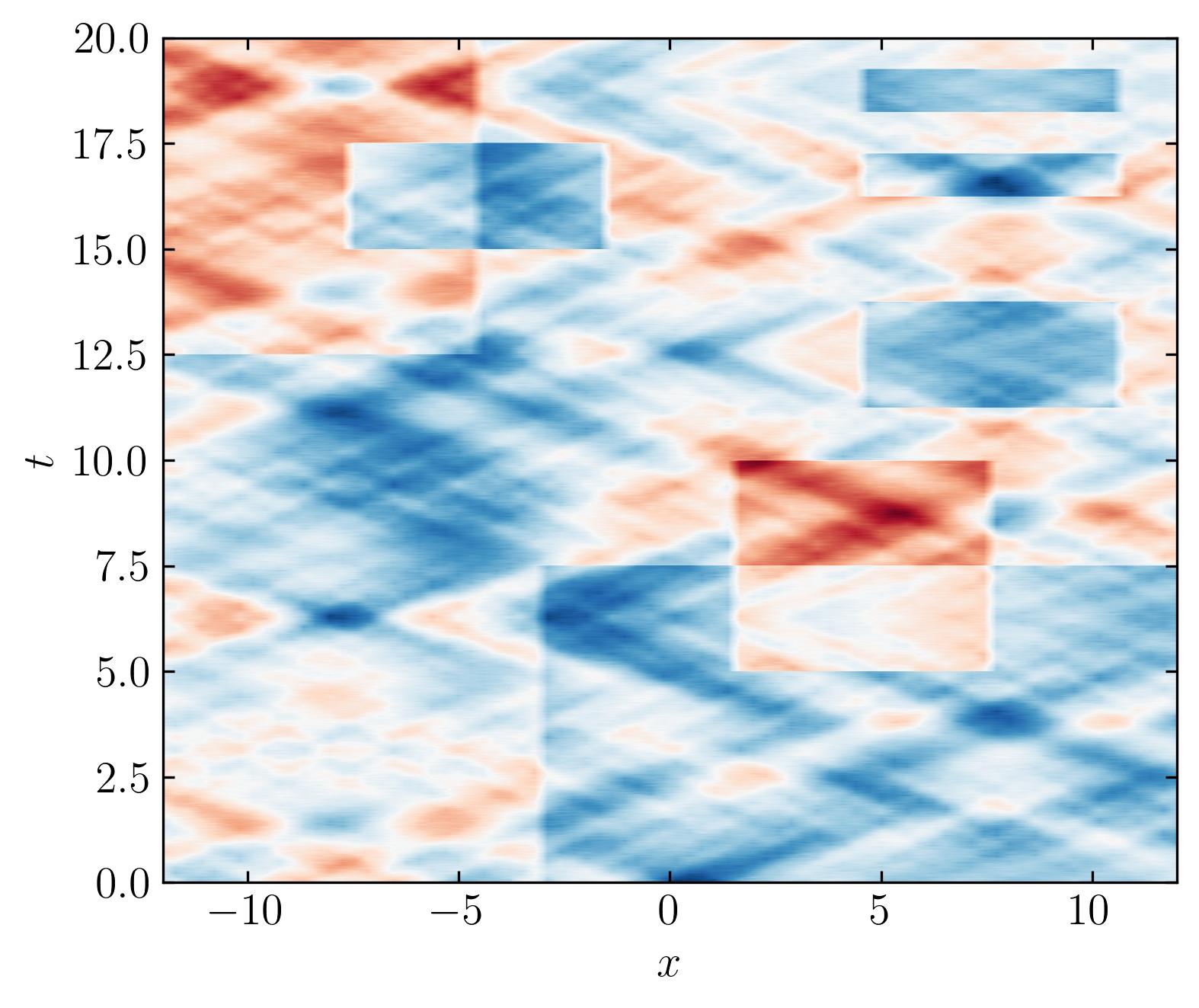
This dataset contains various features spanning multiple time scales. Some features are oscillating sines and cosines, while others are unpredictable, one-time events. The data is entirely synthetic and has no real-world relevance. Before diving into analysis, it’s important to take a quick look at the dataset’s singular values. For this, we’ll use the Optimal Singular Value Hard Threshold (OSVHT) method, proposed by Gavish and Donoho (2014). OSVHT offers a systematic, automatic way to determine the rank of a dataset, eliminating the need for subjective judgment while ensuring optimal dimensionality reduction. The Python implementation of the OSVHT function is as follows:

def svht(X, sv=None):
    # svht for sigma unknown
    m,n = sorted(X.shape) # ensures m <= n
    beta = m / n # ratio between 0 and 1
    if sv is None:
        sv = svdvals(X)
    sv = np.squeeze(sv)
    omega_approx = 0.56 * beta**3 - 0.95 * beta**2 + 1.82 * beta + 1.43
    return np.median(sv) * omega_approx

Let’s pass the X matrix to this function and plot the singular values of the dataset:

# determine rank-reduction
sv = svdvals(X)
tau = svht(X, sv=sv)
r = sum(sv > tau)

# Plot the singular values 
fig, ax = plt.subplots()
ax.plot(sv, 'o', color = 'k')
ax.axhline(tau, color = 'r', linestyle = '--')
ax.xaxis.set_tick_params(direction='in', which='both')
ax.yaxis.set_tick_params(direction='in', which='both')
ax.xaxis.set_ticks_position('both')
ax.yaxis.set_ticks_position('both')
ax.set_xlabel(r'$x$')
ax.set_ylabel(r'$t$')
plt.show()

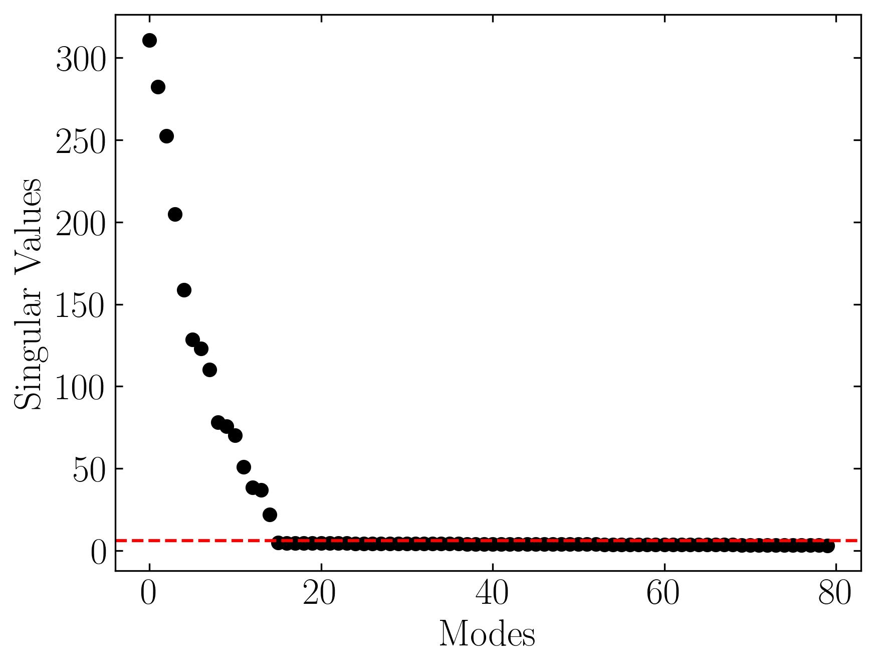
In this plot, the red line represents the optimal cut-off point, or singular value hard threshold (SVHT). This threshold provides a single value that determines the optimal rank for dimensionality reduction. It effectively separates the true modes—those that represent the signal—from the noisy, irrelevant modes. By applying this optimal threshold, we can truncate the singular value decomposition (SVD) and reconstruct a denoised version of the data matrix. The resulting matrix retains the essential structure while removing noise and irregularities.

Now, let’s apply DMD to this dataset.

def dmd(X, Y, truncate=None):
    if truncate == 0:
        # return empty vectors
        mu = np.array([], dtype='complex')
        Phi = np.zeros([X.shape[0], 0], dtype='complex')
    else:
        U2,Sig2,Vh2 = svd(X, False) # SVD of input matrix
        r = len(Sig2) if truncate is None else truncate # rank truncation
        U = U2[:,:r]
        Sig = diag(Sig2)[:r,:r]
        V = Vh2.conj().T[:,:r]
        Atil = dot(dot(dot(U.conj().T, Y), V), inv(Sig)) # build A tilde
        mu,W = eig(Atil)
        Phi = dot(dot(dot(Y, V), inv(Sig)), W) # build DMD modes
    return mu, Phi

Now, let’s compute the DMD:

# Perform DMD
mu,Phi = dmd(X, Y, r)

# Compute time-evolution
b = dot(pinv(Phi), X[:,0])
Vand = np.vander(mu, len(t), True)
Psi = (Vand.T * b).T

# Reconstruct data
D_dmd = dot(Phi, Psi)

Next, let’s plot the reconstructed DMD and see the results:

fig, ax = plt.subplots()
p = ax.contourf(x, t, D_dmd.T, levels = 501, cmap = 'RdBu')
ax.xaxis.set_tick_params(direction='in', which='both')
ax.yaxis.set_tick_params(direction='in', which='both')
ax.xaxis.set_ticks_position('both')
ax.yaxis.set_ticks_position('both')
ax.set_aspect('equal')
ax.set_xlabel(r'$x$')
ax.set_ylabel(r'$t$')
plt.show()

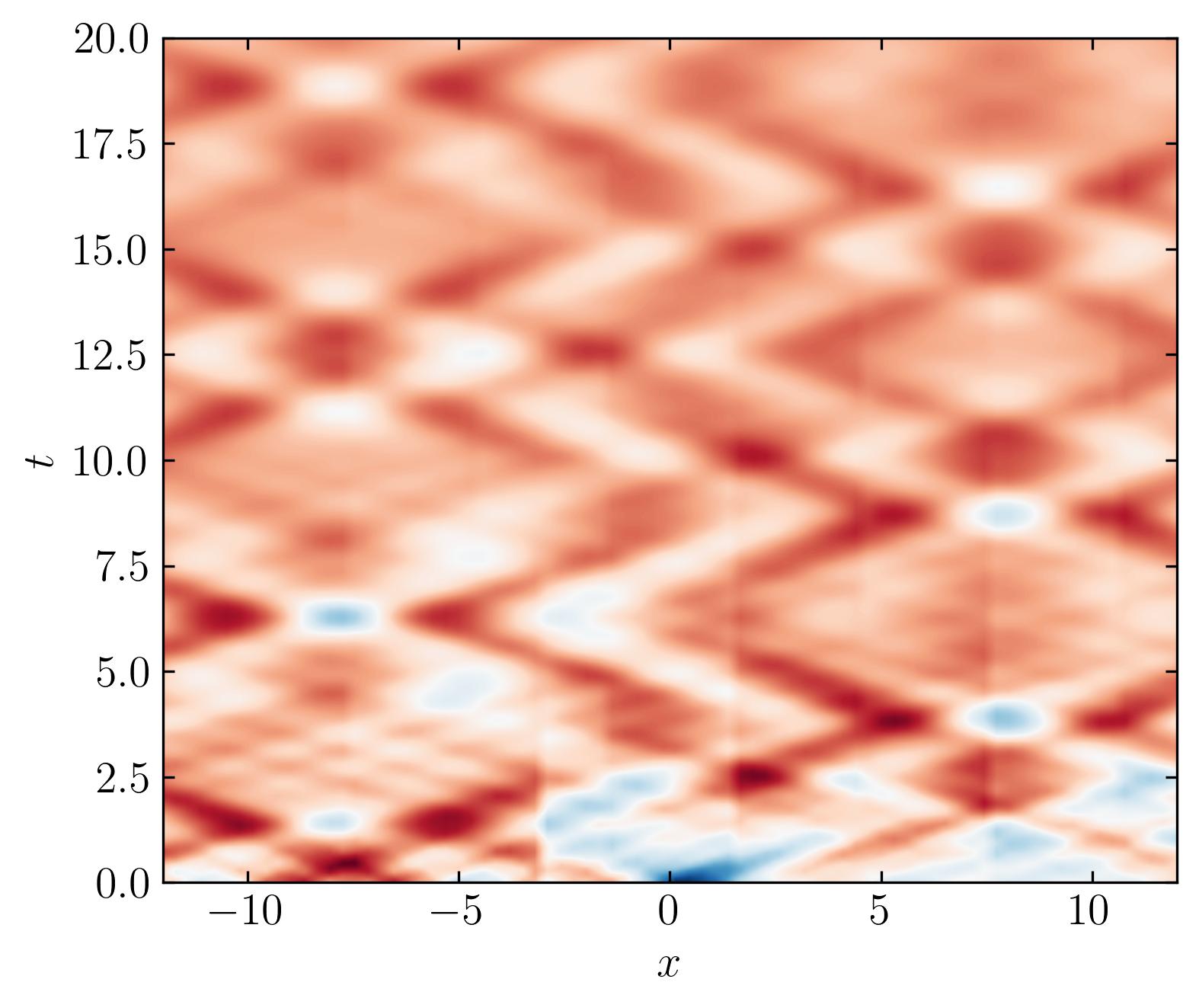
Looking at this reconstruction, it’s clear that DMD fails to capture the original dataset effectively. While some features are represented, the transient events are completely missed. This limitation is significant, but fortunately, it can be addressed using Multi-Resolution Dynamic Mode Decomposition (MRDMD).

MRDMD : The concept

Let’s revisit the basics of DMD discussed in my previous post. Each DMD mode is associated with a relative frequency and a decay/growth rate determined by its eigenvalue ($\Lambda$).

These values can be interpreted as the speed of each DMD mode, where a fast mode oscillates, decays, or grows rapidly, while a slow mode oscillates, decays, or grows slowly. Recall that the time dynamics of a mode are governed by the following equation:

\[\omega_k = ln(\lambda_k)/\Delta t\]

The approximated solution for future times is then:

\[x(t) \approx \sum_{k=1}^r \phi_k e^{\omega_k t}b_k = \Phi e^{\Omega t} b\]

In these equations, the speed of a mode (i.e., the rate at which it decays or grows) is proportional to the natural logarithm of the absolute value of the eigenvalue ($\Lambda$). The exact speed depends on the time units and the sampling rate of the data. A mode is considered slow when it has low frequency or slow growth/decay rates—essentially, it changes gradually as the system evolves over time.

For example, consider the figure below from a DMD analysis of flow past a square cylinder.

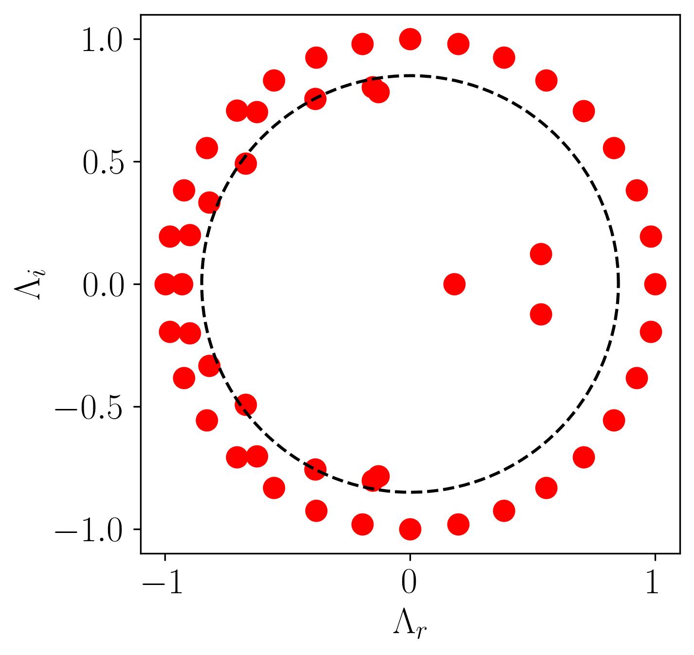
In this plot, a dotted circle of arbitrary radius illustrates the distinction between slow and fast DMD modes. The slow modes are within the circle, exhibiting low growth/decay rates and low frequencies, while the fast modes lie outside the circle.

In the MRDMD algorithm, we recursively extract the slow modes at each time scale, subtracting the slow-mode approximation from the dataset. We then split the dataset in half and repeat the procedure for both halves. This recursive process can be seen as applying DMD to sub-sampled datasets. To improve execution time, we subsample the data at each recursion level, reducing its size to the minimum required to capture slow modes.

Additionally, at each level, we perform rank-reduction using the OSVHT method to determine the optimal cut-off between slow and fast modes. The optimal DMD approximation requires calculating the b vector using the Sparsity-Promoting DMD procedure. Once we obtain the optimal b vector, we can construct a slow-mode approximation to the data. This approximation is then subtracted from the data at the current level to produce a new dataset for the next recursion level.

A python implementation of the MRDMD code, borrowed from HumaticLabs is given below:

def mrdmd(D, level=0, bin_num=0, offset=0, max_levels=7, max_cycles=2, do_svht=True):
    """Compute the multi-resolution DMD on the dataset `D`, returning a list of nodes
    in the hierarchy. Each node represents a particular "time bin" (window in time) at
    a particular "level" of the recursion (time scale). The node is an object consisting
    of the various data structures generated by the DMD at its corresponding level and
    time bin. The `level`, `bin_num`, and `offset` parameters are for record keeping 
    during the recursion and should not be modified unless you know what you are doing.
    The `max_levels` parameter controls the maximum number of levels. The `max_cycles`
    parameter controls the maximum number of mode oscillations in any given time scale 
    that qualify as "slow". The `do_svht` parameter indicates whether or not to perform
    optimal singular value hard thresholding."""

    # 4 times nyquist limit to capture cycles
    nyq = 8 * max_cycles

    # time bin size
    bin_size = D.shape[1]
    if bin_size < nyq:
        return []

    # extract subsamples 
    step = floor(bin_size / nyq) # max step size to capture cycles
    _D = D[:,::step]
    X = _D[:,:-1]
    Y = _D[:,1:]

    # determine rank-reduction
    if do_svht:
        _sv = svdvals(_D)
        tau = svht(_D, sv=_sv)
        r = sum(_sv > tau)
    else:
        r = min(X.shape)

    # compute dmd
    mu,Phi = dmd(X, Y, r)

    # frequency cutoff (oscillations per timestep)
    rho = max_cycles / bin_size

    # consolidate slow eigenvalues (as boolean mask)
    slow = (np.abs(np.log(mu) / (2 * pi * step))) <= rho
    n = sum(slow) # number of slow modes

    # extract slow modes (perhaps empty)
    mu = mu[slow]
    Phi = Phi[:,slow]

    if n > 0:

        # vars for the objective function for D (before subsampling)
        Vand = np.vander(power(mu, 1/step), bin_size, True)
        P = multiply(dot(Phi.conj().T, Phi), np.conj(dot(Vand, Vand.conj().T)))
        q = np.conj(diag(dot(dot(Vand, D.conj().T), Phi)))

        # find optimal b solution
        b_opt = solve(P, q).squeeze()

        # time evolution
        Psi = (Vand.T * b_opt).T

    else:

        # zero time evolution
        b_opt = np.array([], dtype='complex')
        Psi = np.zeros([0, bin_size], dtype='complex')

    # dmd reconstruction
    D_dmd = dot(Phi, Psi)   

    # remove influence of slow modes
    D = D - D_dmd

    # record keeping
    node = type('Node', (object,), {})()
    node.level = level            # level of recursion
    node.bin_num = bin_num        # time bin number
    node.bin_size = bin_size      # time bin size
    node.start = offset           # starting index
    node.stop = offset + bin_size # stopping index
    node.step = step              # step size
    node.rho = rho                # frequency cutoff
    node.r = r                    # rank-reduction
    node.n = n                    # number of extracted modes
    node.mu = mu                  # extracted eigenvalues
    node.Phi = Phi                # extracted DMD modes
    node.Psi = Psi                # extracted time evolution
    node.b_opt = b_opt            # extracted optimal b vector
    nodes = [node]

    # split data into two and do recursion
    if level < max_levels:
        split = ceil(bin_size / 2) # where to split
        nodes += mrdmd(
            D[:,:split],
            level=level+1,
            bin_num=2*bin_num,
            offset=offset,
            max_levels=max_levels,
            max_cycles=max_cycles,
            do_svht=do_svht
            )
        nodes += mrdmd(
            D[:,split:],
            level=level+1,
            bin_num=2*bin_num+1,
            offset=offset+split,
            max_levels=max_levels,
            max_cycles=max_cycles,
            do_svht=do_svht
            )

    return nodes

# Stitch together function
def stitch(nodes, level):
    
    # get length of time dimension
    start = min([nd.start for nd in nodes])
    stop = max([nd.stop for nd in nodes])
    t = stop - start

    # extract relevant nodes
    nodes = [n for n in nodes if n.level == level]
    nodes = sorted(nodes, key=lambda n: n.bin_num)
    
    # stack DMD modes
    Phi = np.hstack([n.Phi for n in nodes])
    
    # allocate zero matrix for time evolution
    nmodes = sum([n.n for n in nodes])
    Psi = np.zeros([nmodes, t], dtype='complex')
    
    # copy over time evolution for each time bin
    i = 0
    for n in nodes:
        _nmodes = n.Psi.shape[0]
        Psi[i:i+_nmodes,n.start:n.stop] = n.Psi
        i += _nmodes
    
    return Phi,Psi

This code returns a list of nodes, each corresponding to a particular time scale and time window. The deeper the recursion (i.e., the higher the level), the finer the time scales and the smaller the time windows. The lowest levels contain only one time window with coarser time scales, while the higher levels consist of many non-overlapping, smaller time windows that capture finer details. Using the stitch command, we can extract all DMD modes and time evolutions from a given level into a single pair of $\Phi$ and $\Psi$ matrices.

Let’s compute MRDMD now:

# Compute MRDMD
nodes = mrdmd(D)

# stitch modes
Phi0,Psi0 = stitch(nodes, 0) # slow modes
Phi1,Psi1 = stitch(nodes, 1) # fast modes 
Phi2,Psi2 = stitch(nodes, 2) # faster modes
Phi3,Psi3 = stitch(nodes, 3)
Phi4,Psi4 = stitch(nodes, 4)
Phi5,Psi5 = stitch(nodes, 5)
Phi6,Psi6 = stitch(nodes, 6)

Next, let’s visualize the DMD modes and their time evolution for slow, fast, and faster modes:

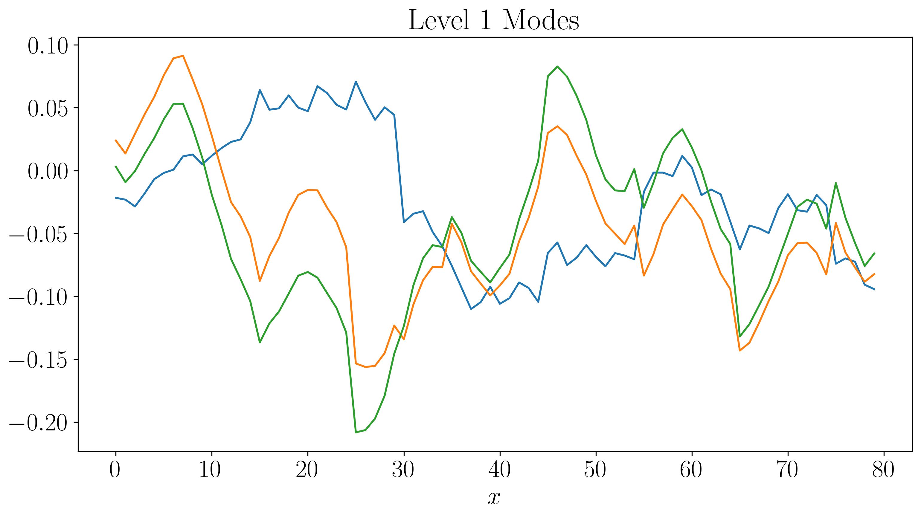
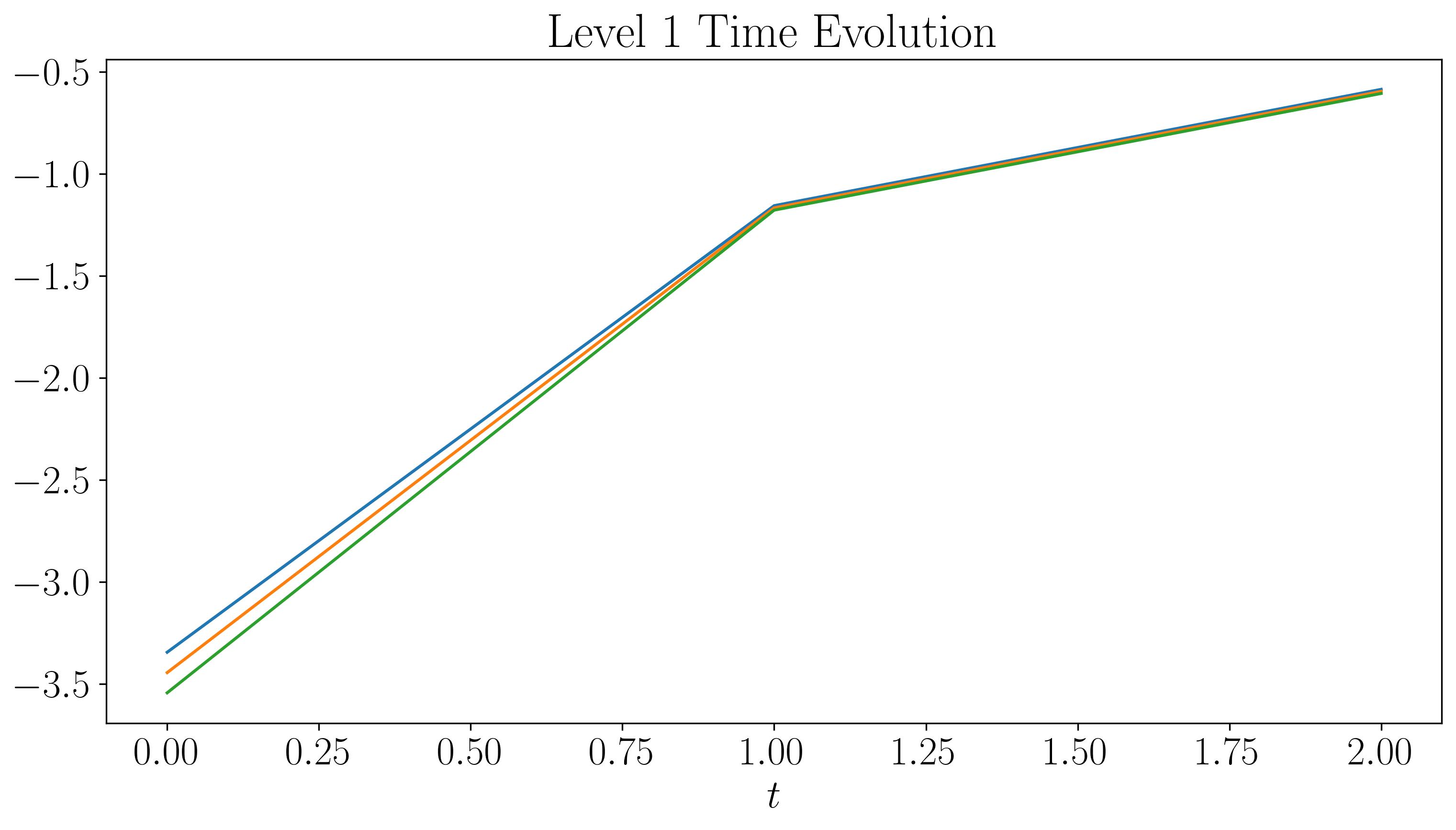
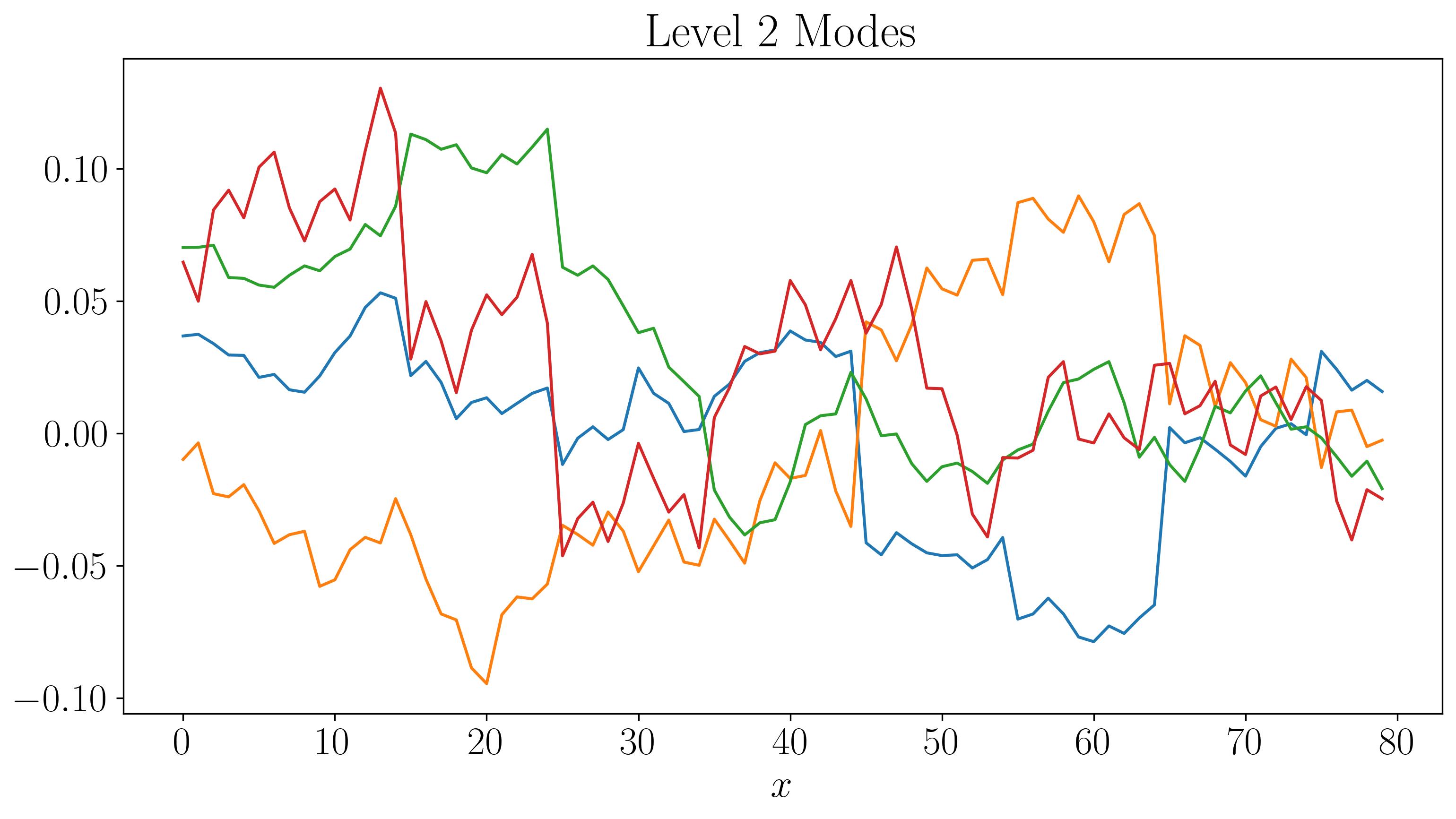
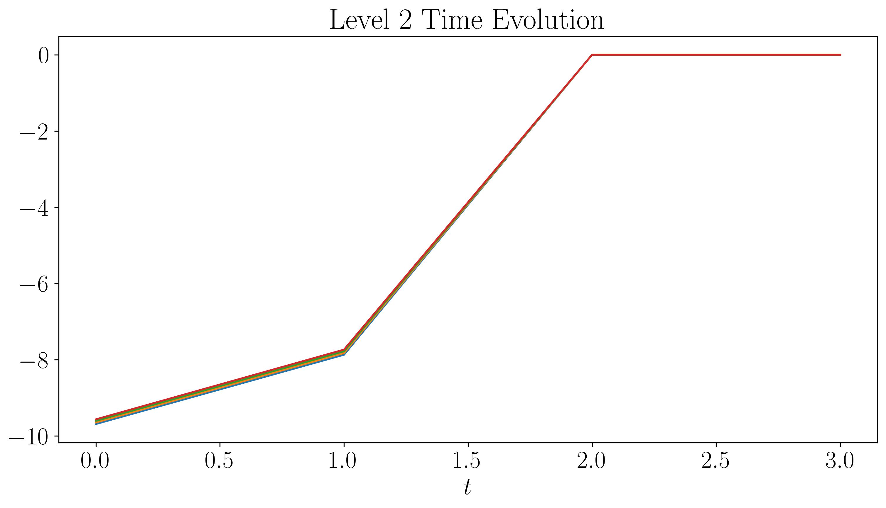
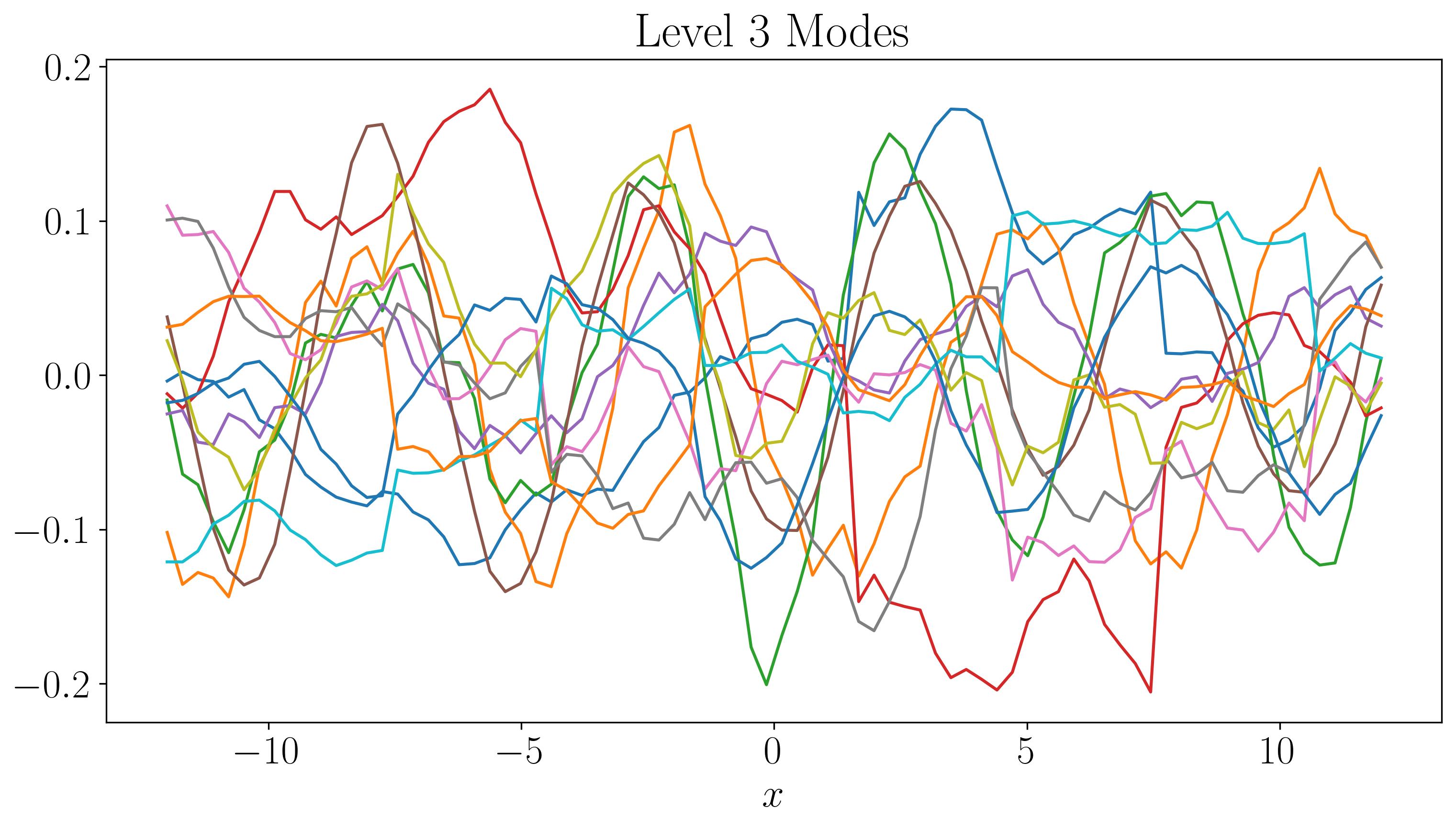
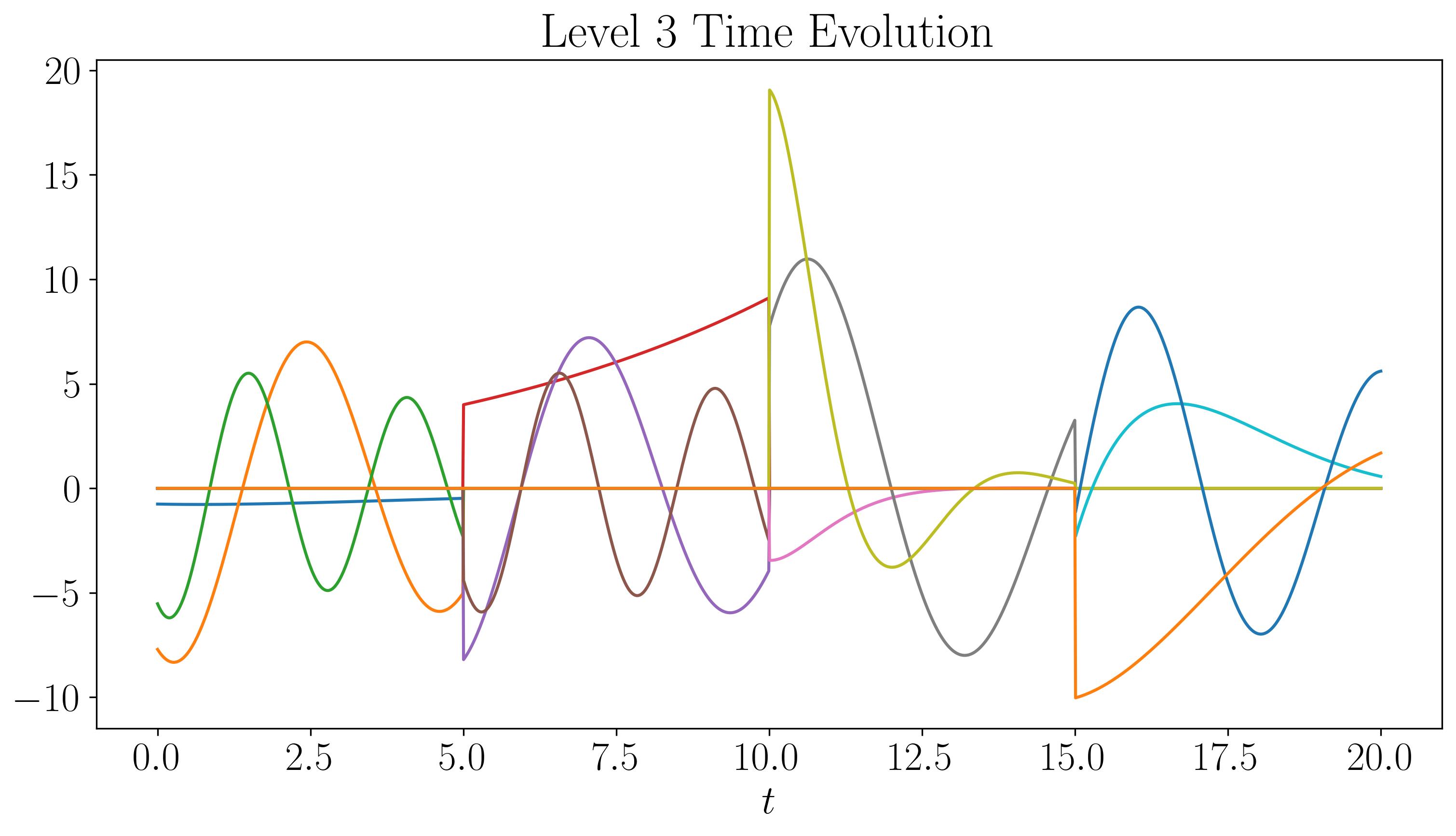
For the first two levels, the modes look similar to those generated by a single application of DMD. While there are some discontinuities in the modes and time evolution, they are not highly pronounced. At the third level, the plots start filling up quickly. As we go to higher levels, we begin to observe finer discontinuities in both space and time, closely resembling the original dataset.

Now, let’s visualize the reconstruction of the MRDMD-approximated datasets at each level. For each level, starting with the first, we will construct an approximation of the data at the corresponding time scale.

D_mrdmd = [dot(*stitch(nodes, i)) for i in range(7)]

First, let’s visualize the MRDMD reconstructions at each level:

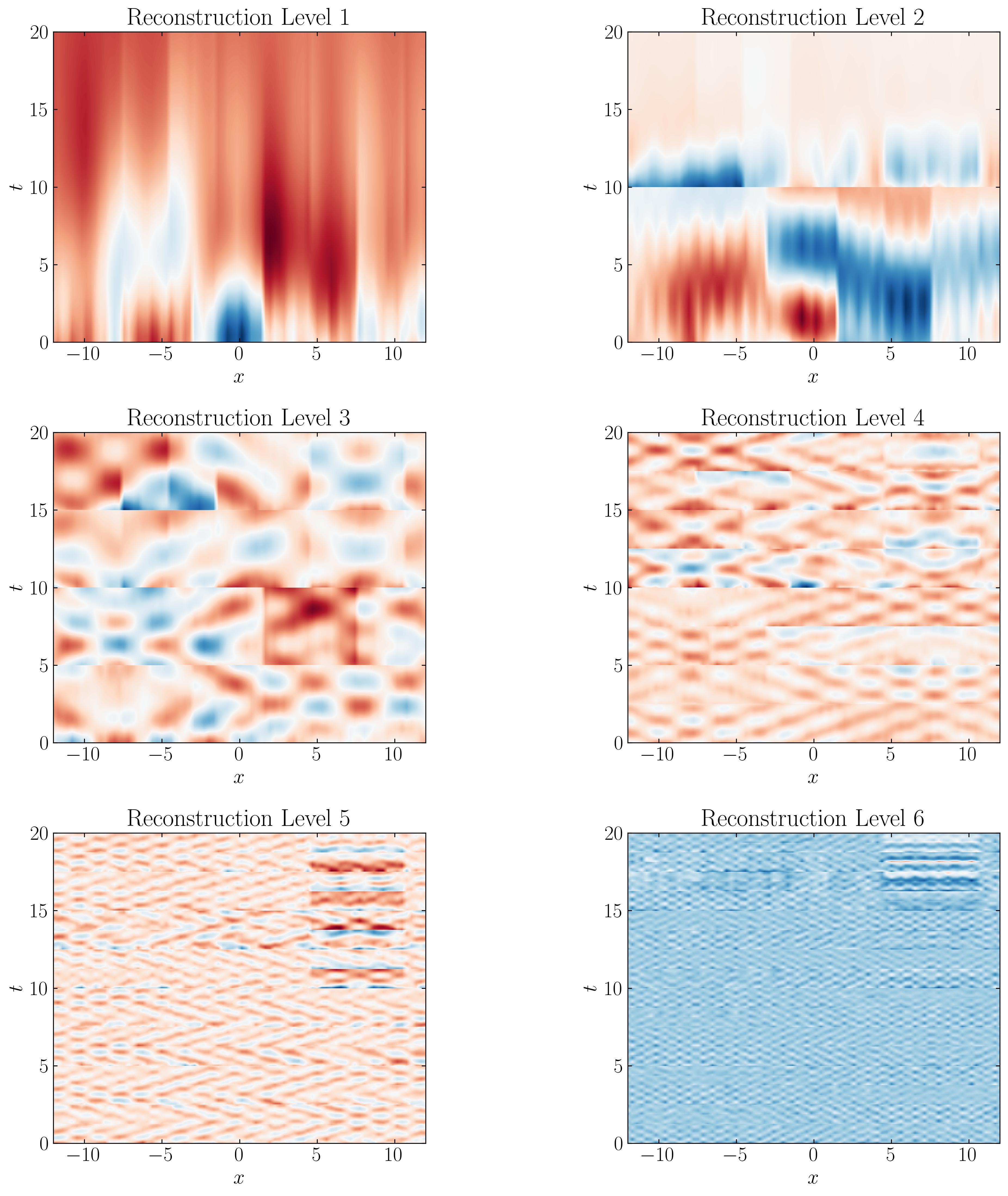
We can observe that the approximation at each level captures progressively finer time scales. For example, the Level 7 reconstruction reveals the finest structures corresponding to the smallest time scales in the dataset, which are essentially the noise. It’s fascinating to see how the original data has been broken down into components at increasingly fine resolutions.

Now, let’s sequentially combine the reconstructions from each level and attempt to approximate the original dataset. For reference, here’s how you can plot the reconstructions:

fig, ax = plt.subplots()
p = ax.contourf(x, t, D_mrdmd[0].T+D_mrdmd[1].T, levels = 501, cmap = 'RdBu')
ax.xaxis.set_tick_params(direction='in', which='both')
ax.yaxis.set_tick_params(direction='in', which='both')
ax.xaxis.set_ticks_position('both')
ax.yaxis.set_ticks_position('both')
ax.set_aspect('equal')
ax.set_xlabel(r'$x$')
ax.set_ylabel(r'$t$')
ax.set_title('Sum to Level 2')
plt.show()

Here are the results:

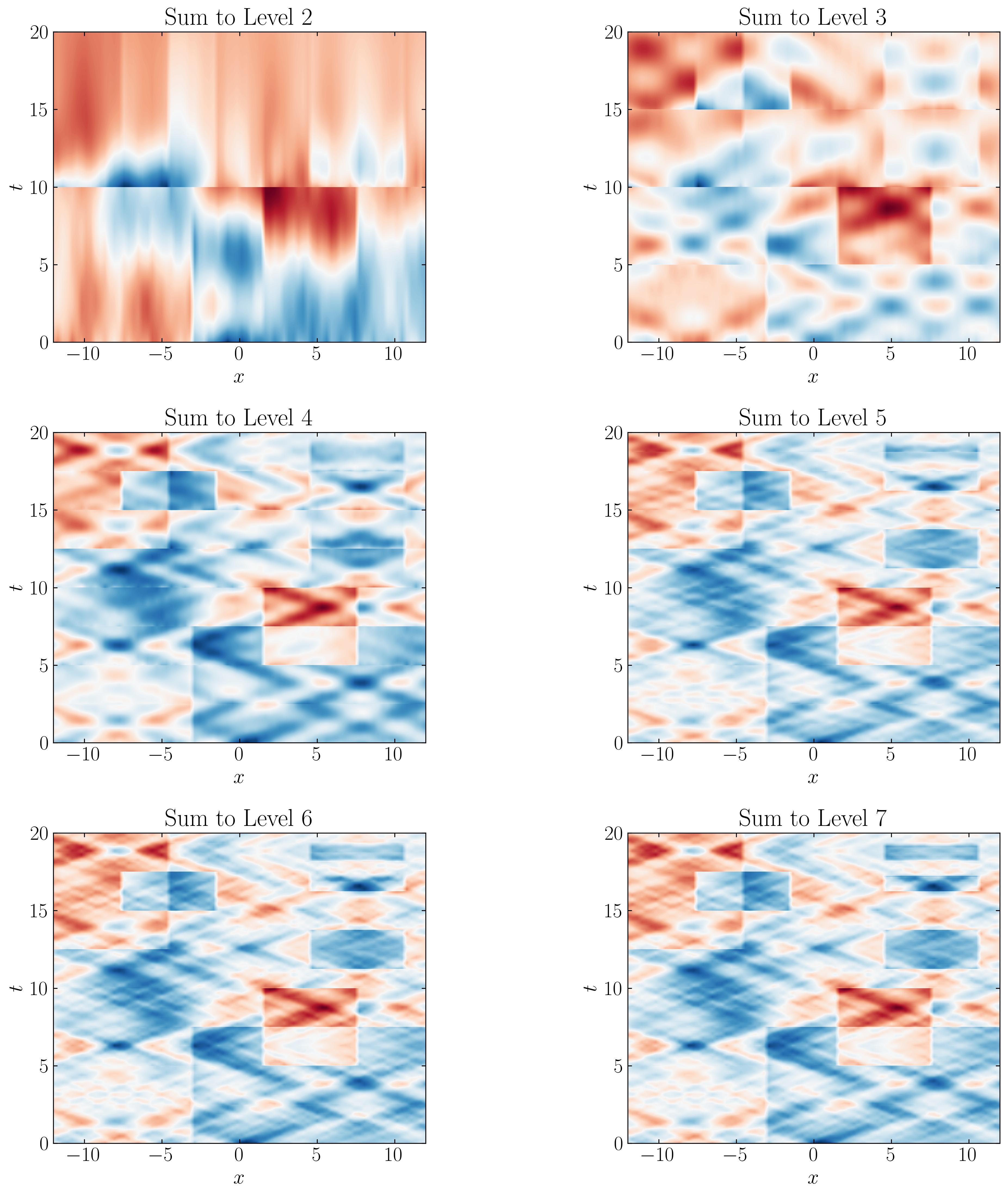
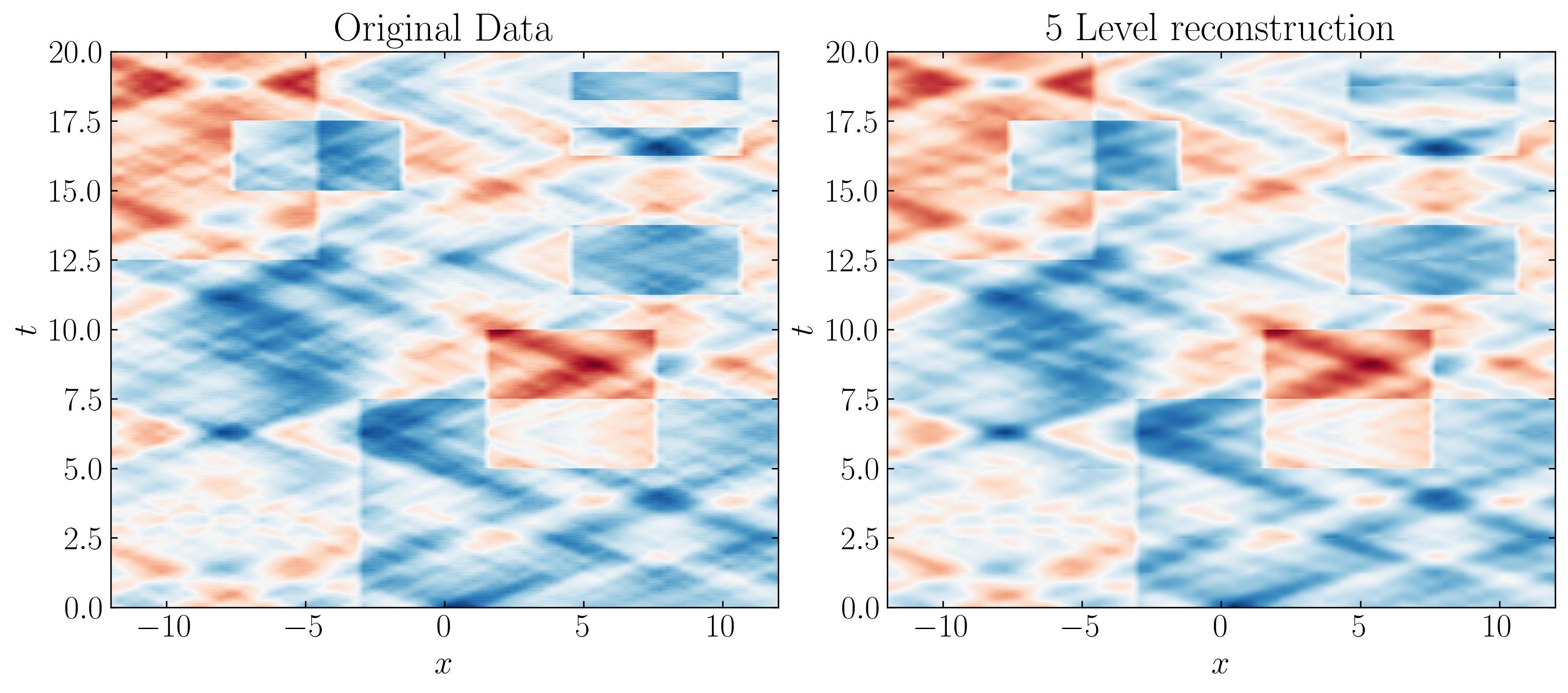
As we progress through each level, the DMD approximation captures finer temporal behaviors, more closely resembling the original dataset. Comparing these side by side with the original dataset, we can observe that a Level 5 reconstruction is sufficient to capture the minute details of the original data.

In conclusion, the power of MRDMD shines through in this tutorial, showcasing its remarkable versatility and ease of use. For one, it’s entirely self-contained, no fiddling with parameters is required. But what truly sets MRDMD apart is its ability to capture the intricate dynamics of data at multiple resolutions. Whether you’re analyzing long-term trends, medium-term patterns, or short-term fluctuations, MRDMD provides a systematic, multi-layered approach to uncovering these features. It handles transient phenomena with finesse, seamlessly removing noise while preserving essential structures (especially when paired with the optimal SVHT). Most importantly, MRDMD is not just efficient but adaptable, making it a powerful tool across a diverse array of fields-from physics and biology to finance and beyond.