Data-Driven Modal Analysis with MODULO and OpenFOAM
In recent years, data-driven modal decomposition has become an essential tool in fluid dynamics research, offering a powerful means to distill complex flow dynamics into meaningful patterns. In this blog, I’ll introduce MODULO, a versatile software developed at the von Karman Institute for Fluid Dynamics specifically for this purpose. MODULO is designed to make sophisticated decomposition techniques, like Proper Orthogonal Decomposition (POD) and Dynamic Mode Decomposition (DMD), accessible and highly effective, especially when working with large datasets from computational tools like OpenFOAM.

As my series of articles on data-driven modal decomposition wraps up, I’m excited to share one last tool in the data-driven modal analysis toolbox for Python users: MODULO, or MODal mULtiscale pOd. Developed at the von Karman Institute for Fluid Dynamics, MODULO is an advanced software designed to perform a range of powerful data-driven decompositions. Originally created for Multiscale Proper Orthogonal Decomposition (mPOD), it now supports an impressive suite of methods, including POD, SPOD, DFT, DMD, and more. What sets MODULO apart is its efficiency—it’s optimized for handling large datasets through a memory-saving feature that divides the data into manageable chunks, making it ideal for complex applications. Plus, it can handle non-uniform meshes with precision, thanks to its weighted inner product approach. Although MODULO relies on NumPy routines and doesn’t yet have additional parallel computing features, its efficiency in processing is impressive.
MODULO currently offers the following decompositions:
- Discrete Fourier Transform (DFT) by Briggs et al. (1995)
- Proper Orthogonal Decomposition (POD) by Berkooz et al. (1993)
- Multi-Scale Proper Orthogonal Decomposition (mPOD) by Mendez et al. (2019)
- Dynamic Mode Decomposition (DMD) by Schmid (2010)
- Spectral Proper Orthogonal Decomposition (SPOD) by Towne et al. (2018)
- Spectral Proper Orthogonal Decomposition (SPOD) by Sieber et al. (2016)
- Kernel Proper Orthogonal Decomposition (KPOD) by Mika et al. (1998)
In this article, I’ll guide you through how to apply POD and DMD using the MODULO package with OpenFOAM simulation data.
Lets Begin!!
Installing MODULO
Getting started with MODULO is straightforward. The package is available on PyPI, and you can install it with a single command:
pip install modulo_vki
Before you proceed, ensure that you have the following dependencies installed, as they are essential for MODULO’s functionality:
pip install tqdm numpy scipy scikit-learn ipykernel ipython ipython-genutils ipywidgets matplotlib pyvista imageio
Precursor steps
To get started, open a Jupyter notebook and import the necessary libraries and modules:
import matplotlib.colors
import matplotlib.pyplot as plt
import numpy as np
import pandas as pd
import fluidfoam as fl
import scipy as sp
import os
import matplotlib.animation as animation
import pyvista as pv
from modulo_vki import ModuloVKI # this is to create modulo objects
import imageio
import io
%matplotlib inline
plt.rcParams.update({'font.size' : 18, 'font.family' : 'Times New Roman', "text.usetex": True})

# Path variables
Path = 'E:/Blog_Posts/Simulations/Sq_Cyl_Surfaces/surfaces/'
save_path = 'E:/Blog_Posts/OpenFOAM/ROM_Series/Post40/'
In previous articles, I demonstrated how to extract snapshot data from an OpenFOAM simulation using surface data. For a detailed guide, refer to my earlier article.
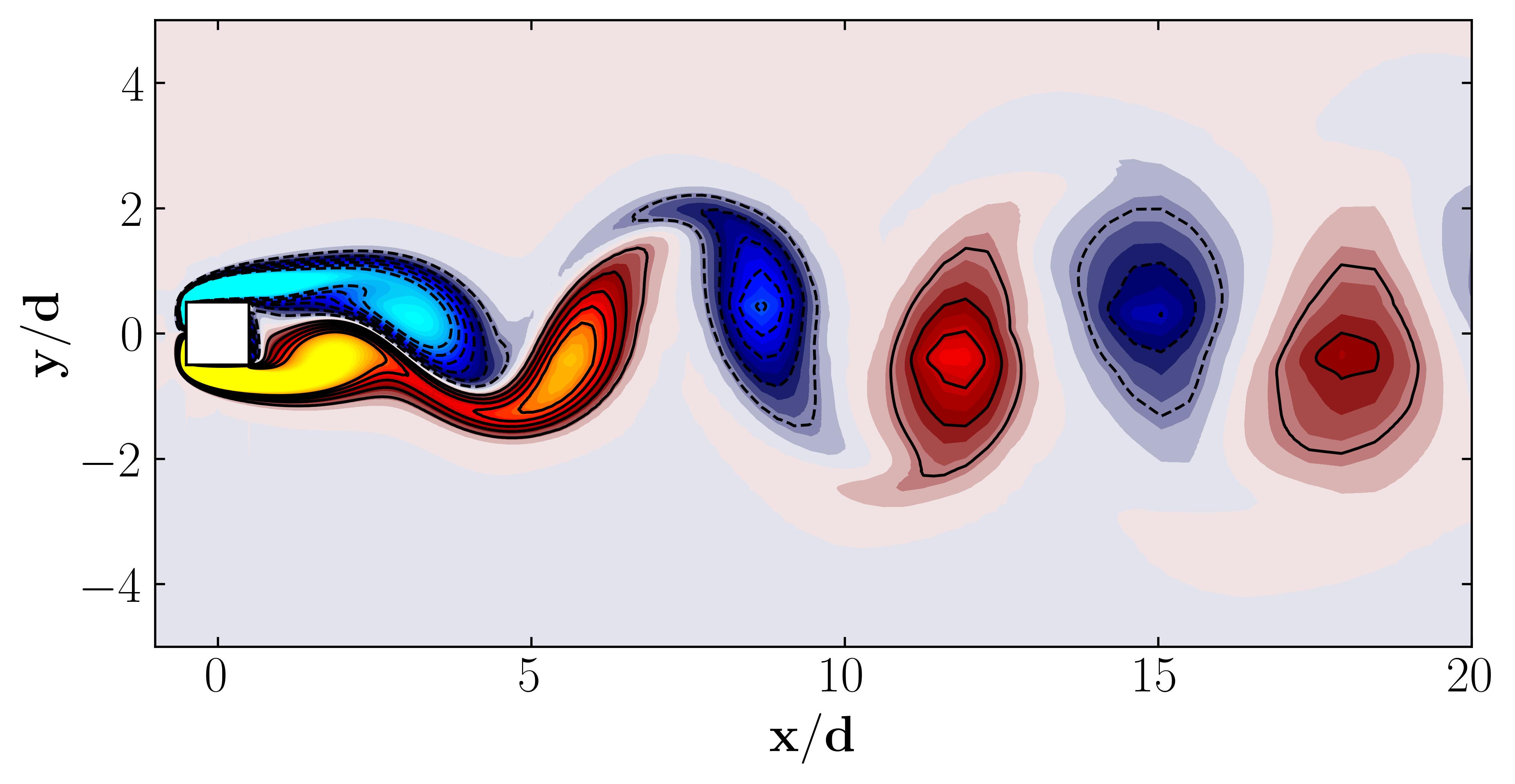
In this tutorial, I’ll be using a dataset from a flow simulation around a square cylinder at a Reynolds number of 100, computed with Direct Numerical Simulations (DNS) in OpenFOAM. The setup closely follows the configuration outlined by Bai and Alam (2018).
Here, we’ll use vorticity data from my previous tutorials. Load the vorticity snapshot matrix as follows:
# Vorticity snapshot matrix
data_Vort = np.load(save_path + 'VortZ.npy')

# Grid information for plotting
Files = os.listdir(Path)
Data = pv.read(Path + Files[0] + '/zNormal.vtp')
grid = Data.points
x = grid[:,0]
y = grid[:,1]
z = grid[:,2]
rows, columns = np.shape(grid)
print('rows = ', rows, 'columns = ', columns)

# Constants
d = 0.1
Ub = 0.015
For reference, here’s what the vorticity dataset looks like:
Performing Proper Orthogonal Decomposition (POD) Using MODULO
To start, let’s calculate the Proper Orthogonal Decomposition (POD) of the dataset using the MODULO package.
# --- Initialize MODULO object
m2 = ModuloVKI(data=np.nan_to_num(data_Vort), n_Modes=50)

# POD via svd
Phi_P, Psi_P, Sigma_P = m2.compute_POD_svd()

# OR Compute the POD using Sirovinch's method
Phi_POD, Psi_POD, Sigma_POD = m2.compute_POD_K()
MODULO provides two approaches for computing POD:
- Snapshot Method (using temporal correlation matrix) - This approach works well for high-dimensional data.
- Singular Value Decomposition (SVD) - A more general approach for smaller datasets.
For consistency with my previous articles, I’ll be using the Method of Snapshots, which can efficiently handle large datasets and capture the dominant flow structures.
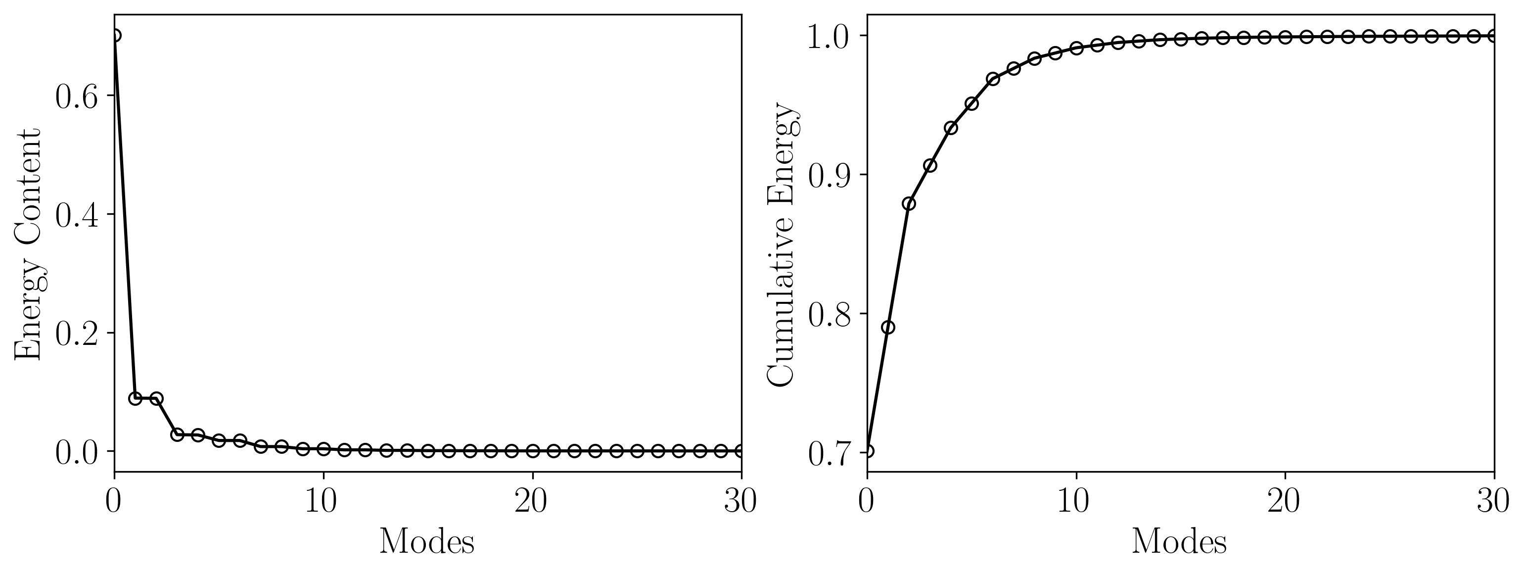
Next, let’s visualize the energy content of each POD mode along with the cumulative energy to understand the distribution:
Energy = np.zeros((len(Sigma_P),1))
for i in np.arange(0,len(Sigma_P)):
    Energy[i] = Sigma_P[i]/np.sum(Sigma_P)

X_Axis = np.arange(Energy.shape[0])
heights = Energy[:,0]

fig, axes = plt.subplots(1, 2, figsize = (12,4))
ax = axes[0]
ax.plot(Energy, marker = 'o', markerfacecolor = 'none', markeredgecolor = 'k', ls='-', color = 'k')
ax.set_xlim(0, 30)
ax.set_xlabel('Modes')
ax.set_ylabel('Energy Content')

ax = axes[1]
cumulative = np.cumsum(Sigma_P)/np.sum(Sigma_P)
ax.plot(cumulative, marker = 'o', markerfacecolor = 'none', markeredgecolor = 'k', ls='-', color = 'k')
ax.set_xlabel('Modes')
ax.set_ylabel('Cumulative Energy')
ax.set_xlim(0, 30)

plt.show()
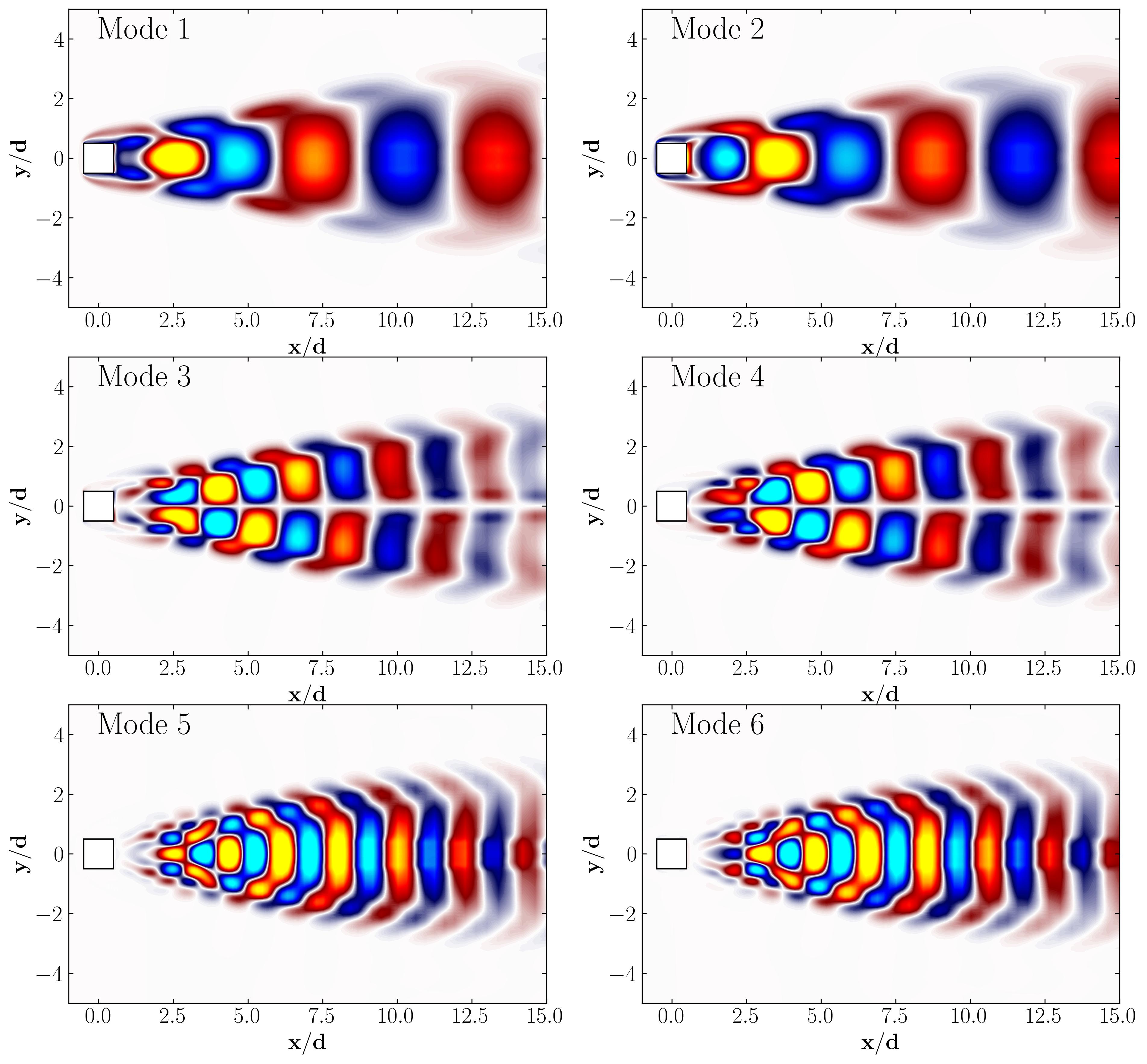
Once the POD has been computed, we can visualize the spatial structures of the individual POD modes. Here’s how to plot the POD modes using matplotlib:
d = 0.1
Ub = 0.015

fig, axs = plt.subplots(3, 2, figsize=(15, 15))

ax = axs[0,0]
Mode = 1
p = ax.tricontourf(x/0.1, y/0.1, Phi_P[:,Mode]*(d/Ub), levels = 501,
                   vmin=-0.1, vmax=0.1, cmap = cmap)
Rect1 = plt.Rectangle((-0.5, -0.5), 1, 1, ec='k', color='white')
ax.add_patch(Rect1)
ax.xaxis.set_tick_params(direction='in', which='both')
ax.yaxis.set_tick_params(direction='in', which='both')
ax.xaxis.set_ticks_position('both')
ax.yaxis.set_ticks_position('both')
ax.set_xlim(-1, 15)
ax.set_ylim(-5, 5)
ax.set_aspect('equal')

ax.set_xlabel(r'$\bf x/d$')
ax.set_ylabel(r'$\bf y/d$')
ax.text(0, 4, 'Mode 1', fontsize = 25, color = 'black')

ax = axs[0,1]
Mode = 2
p = ax.tricontourf(x/0.1, y/0.1, Phi_P[:,Mode]*(d/Ub), levels = 501,
                   vmin=-0.1, vmax=0.1, cmap = cmap)
Rect1 = plt.Rectangle((-0.5, -0.5), 1, 1, ec='k', color='white')
ax.add_patch(Rect1)
ax.xaxis.set_tick_params(direction='in', which='both')
ax.yaxis.set_tick_params(direction='in', which='both')
ax.xaxis.set_ticks_position('both')
ax.yaxis.set_ticks_position('both')
ax.set_xlim(-1, 15)
ax.set_ylim(-5, 5)
ax.set_aspect('equal')

ax.set_xlabel(r'$\bf x/d$')
ax.set_ylabel(r'$\bf y/d$')
ax.text(0, 4, 'Mode 2', fontsize = 25, color = 'black')

ax = axs[1,0]
Mode = 3
p = ax.tricontourf(x/0.1, y/0.1, Phi_P[:,Mode]*(d/Ub), levels = 501,
                   vmin=-0.1, vmax=0.1, cmap = cmap)
Rect1 = plt.Rectangle((-0.5, -0.5), 1, 1, ec='k', color='white')
ax.add_patch(Rect1)
ax.xaxis.set_tick_params(direction='in', which='both')
ax.yaxis.set_tick_params(direction='in', which='both')
ax.xaxis.set_ticks_position('both')
ax.yaxis.set_ticks_position('both')
ax.set_xlim(-1, 15)
ax.set_ylim(-5, 5)
ax.set_aspect('equal')

ax.set_xlabel(r'$\bf x/d$')
ax.set_ylabel(r'$\bf y/d$')
ax.text(0, 4, 'Mode 3', fontsize = 25, color = 'black')

ax = axs[1,1]
Mode = 4
p = ax.tricontourf(x/0.1, y/0.1, Phi_P[:,Mode]*(d/Ub), levels = 501,
                   vmin=-0.1, vmax=0.1, cmap = cmap)
Rect1 = plt.Rectangle((-0.5, -0.5), 1, 1, ec='k', color='white')
ax.add_patch(Rect1)
ax.xaxis.set_tick_params(direction='in', which='both')
ax.yaxis.set_tick_params(direction='in', which='both')
ax.xaxis.set_ticks_position('both')
ax.yaxis.set_ticks_position('both')
ax.set_xlim(-1, 15)
ax.set_ylim(-5, 5)
ax.set_aspect('equal')

ax.set_xlabel(r'$\bf x/d$')
ax.set_ylabel(r'$\bf y/d$')
ax.text(0, 4, 'Mode 4', fontsize = 25, color = 'black')

ax = axs[2,0]
Mode = 5
p = ax.tricontourf(x/0.1, y/0.1, Phi_P[:,Mode]*(d/Ub), levels = 501,
                   vmin=-0.1, vmax=0.1, cmap = cmap)
Rect1 = plt.Rectangle((-0.5, -0.5), 1, 1, ec='k', color='white')
ax.add_patch(Rect1)
ax.xaxis.set_tick_params(direction='in', which='both')
ax.yaxis.set_tick_params(direction='in', which='both')
ax.xaxis.set_ticks_position('both')
ax.yaxis.set_ticks_position('both')
ax.set_xlim(-1, 15)
ax.set_ylim(-5, 5)
ax.set_aspect('equal')

ax.set_xlabel(r'$\bf x/d$')
ax.set_ylabel(r'$\bf y/d$')
ax.text(0, 4, 'Mode 5', fontsize = 25, color = 'black')

ax = axs[2,1]
Mode = 6
p = ax.tricontourf(x/0.1, y/0.1, Phi_P[:,Mode]*(d/Ub), levels = 501,
                   vmin=-0.1, vmax=0.1, cmap = cmap)
Rect1 = plt.Rectangle((-0.5, -0.5), 1, 1, ec='k', color='white')
ax.add_patch(Rect1)
ax.xaxis.set_tick_params(direction='in', which='both')
ax.yaxis.set_tick_params(direction='in', which='both')
ax.xaxis.set_ticks_position('both')
ax.yaxis.set_ticks_position('both')
ax.set_xlim(-1, 15)
ax.set_ylim(-5, 5)
ax.set_aspect('equal')

ax.set_xlabel(r'$\bf x/d$')
ax.set_ylabel(r'$\bf y/d$')
ax.text(0, 4, 'Mode 6', fontsize = 25, color = 'black')

fig.subplots_adjust(hspace=0)
plt.show()
Dynamic Mode Decomposition (DMD) with MODULO
Dynamic Mode Decomposition (DMD) is a powerful tool to decompose complex, dynamic data into coherent structures with specific frequencies. Using MODULO, we can compute DMD in a few straightforward steps. Below, we’ll go through setting up DMD, visualizing eigenvalues, and exploring the results.
# time-step and frequency
dt = 0.01*142
F_S = 1/dt

# Compute DMD
Phi_D, Lambda, freqs, a0s = m2.compute_DMD_PIP(False, F_S=F_S)
Plotting the real vs. imaginary parts of the eigenvalues on the unit circle provides insight into the stability of DMD modes. Eigenvalues on or near the unit circle signify neutral modes (neither growing nor decaying), while those inside indicate decay and those outside indicate growth.
fig, ax = plt.subplots()
plt.plot(np.imag(Lambda),np.real(Lambda),'ko')
circle=plt.Circle((0,0),1,color='b', fill=False)
ax.add_patch(circle)
ax.set_aspect('equal')
ax.set_xlabel(r'$\Lambda_r$')
ax.set_ylabel(r'$\Lambda_i$')
plt.tight_layout()
plt.show()
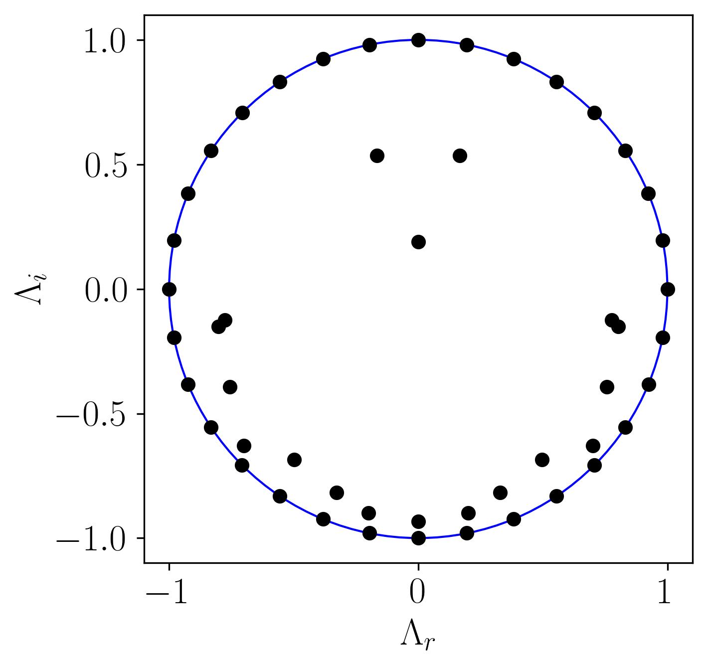
In this plot:
- On the Unit Circle: Indicates stable DMD modes (neither growing nor decaying).
- Inside the Circle: Represents decaying or transient modes.
- Outside the Circle: Denotes modes with growth tendencies, potentially signifying instability.
With DMD, we can visualize the spatial structures and corresponding frequencies of each mode, offering a deeper understanding of flow dynamics. Here’s how you can plot the modes with their frequencies:
d = 0.1
Ub = 0.015

fig, axs = plt.subplots(3, 2, figsize=(15, 15))

ax = axs[0,0]
Mode = 0
p = ax.tricontourf(x/0.1, y/0.1, np.real(Phi_D[:,Mode]*(d/Ub)), levels = 501,
                   vmin=-0.1, vmax=0.1, cmap = cmap)
Rect1 = plt.Rectangle((-0.5, -0.5), 1, 1, ec='k', color='white')
ax.add_patch(Rect1)
ax.xaxis.set_tick_params(direction='in', which='both')
ax.yaxis.set_tick_params(direction='in', which='both')
ax.xaxis.set_ticks_position('both')
ax.yaxis.set_ticks_position('both')
ax.set_xlim(-1, 15)
ax.set_ylim(-5, 5)
ax.set_aspect('equal')

ax.set_xlabel(r'$\bf x/d$')
ax.set_ylabel(r'$\bf y/d$')
ax.text(0, 4, r'$f_i =' + str(freqs[Mode]*(d/Ub)) + '$', fontsize = 25, color = 'black')

ax = axs[0,1]
Mode = 1
p = ax.tricontourf(x/0.1, y/0.1, np.real(Phi_D[:,Mode]*(d/Ub)), levels = 501,
                   vmin=-0.1, vmax=0.1, cmap = cmap)
Rect1 = plt.Rectangle((-0.5, -0.5), 1, 1, ec='k', color='white')
ax.add_patch(Rect1)
ax.xaxis.set_tick_params(direction='in', which='both')
ax.yaxis.set_tick_params(direction='in', which='both')
ax.xaxis.set_ticks_position('both')
ax.yaxis.set_ticks_position('both')
ax.set_xlim(-1, 15)
ax.set_ylim(-5, 5)
ax.set_aspect('equal')

ax.set_xlabel(r'$\bf x/d$')
ax.set_ylabel(r'$\bf y/d$')
ax.text(0, 4, r'$f_i =' + str(freqs[Mode]*(d/Ub)) + '$', fontsize = 25, color = 'black')

ax = axs[1,0]
Mode = 2
p = ax.tricontourf(x/0.1, y/0.1, np.real(Phi_D[:,Mode]*(d/Ub)), levels = 501,
                   vmin=-0.1, vmax=0.1, cmap = cmap)
Rect1 = plt.Rectangle((-0.5, -0.5), 1, 1, ec='k', color='white')
ax.add_patch(Rect1)
ax.xaxis.set_tick_params(direction='in', which='both')
ax.yaxis.set_tick_params(direction='in', which='both')
ax.xaxis.set_ticks_position('both')
ax.yaxis.set_ticks_position('both')
ax.set_xlim(-1, 15)
ax.set_ylim(-5, 5)
ax.set_aspect('equal')

ax.set_xlabel(r'$\bf x/d$')
ax.set_ylabel(r'$\bf y/d$')
ax.text(0, 4, r'$f_i =' + str(freqs[Mode]*(d/Ub)) + '$', fontsize = 25, color = 'black')

ax = axs[1,1]
Mode = 3
p = ax.tricontourf(x/0.1, y/0.1, np.real(Phi_D[:,Mode]*(d/Ub)), levels = 501,
                   vmin=-0.1, vmax=0.1, cmap = cmap)
Rect1 = plt.Rectangle((-0.5, -0.5), 1, 1, ec='k', color='white')
ax.add_patch(Rect1)
ax.xaxis.set_tick_params(direction='in', which='both')
ax.yaxis.set_tick_params(direction='in', which='both')
ax.xaxis.set_ticks_position('both')
ax.yaxis.set_ticks_position('both')
ax.set_xlim(-1, 15)
ax.set_ylim(-5, 5)
ax.set_aspect('equal')

ax.set_xlabel(r'$\bf x/d$')
ax.set_ylabel(r'$\bf y/d$')
ax.text(0, 4, r'$f_i =' + str(freqs[Mode]*(d/Ub)) + '$', fontsize = 25, color = 'black')

ax = axs[2,0]
Mode = 4
p = ax.tricontourf(x/0.1, y/0.1, np.real(Phi_D[:,Mode]*(d/Ub)), levels = 501,
                   vmin=-0.1, vmax=0.1, cmap = cmap)
Rect1 = plt.Rectangle((-0.5, -0.5), 1, 1, ec='k', color='white')
ax.add_patch(Rect1)
ax.xaxis.set_tick_params(direction='in', which='both')
ax.yaxis.set_tick_params(direction='in', which='both')
ax.xaxis.set_ticks_position('both')
ax.yaxis.set_ticks_position('both')
ax.set_xlim(-1, 15)
ax.set_ylim(-5, 5)
ax.set_aspect('equal')

ax.set_xlabel(r'$\bf x/d$')
ax.set_ylabel(r'$\bf y/d$')
ax.text(0, 4, r'$f_i =' + str(freqs[Mode]*(d/Ub)) + '$', fontsize = 25, color = 'black')

ax = axs[2,1]
Mode = 5
p = ax.tricontourf(x/0.1, y/0.1, np.real(Phi_D[:,Mode]*(d/Ub)), levels = 501,
                   vmin=-0.1, vmax=0.1, cmap = cmap)
Rect1 = plt.Rectangle((-0.5, -0.5), 1, 1, ec='k', color='white')
ax.add_patch(Rect1)
ax.xaxis.set_tick_params(direction='in', which='both')
ax.yaxis.set_tick_params(direction='in', which='both')
ax.xaxis.set_ticks_position('both')
ax.yaxis.set_ticks_position('both')
ax.set_xlim(-1, 15)
ax.set_ylim(-5, 5)
ax.set_aspect('equal')

ax.set_xlabel(r'$\bf x/d$')
ax.set_ylabel(r'$\bf y/d$')
ax.text(0, 4, r'$f_i =' + str(freqs[Mode]*(d/Ub)) + '$', fontsize = 25, color = 'black')

fig.subplots_adjust(hspace=0)
plt.show()
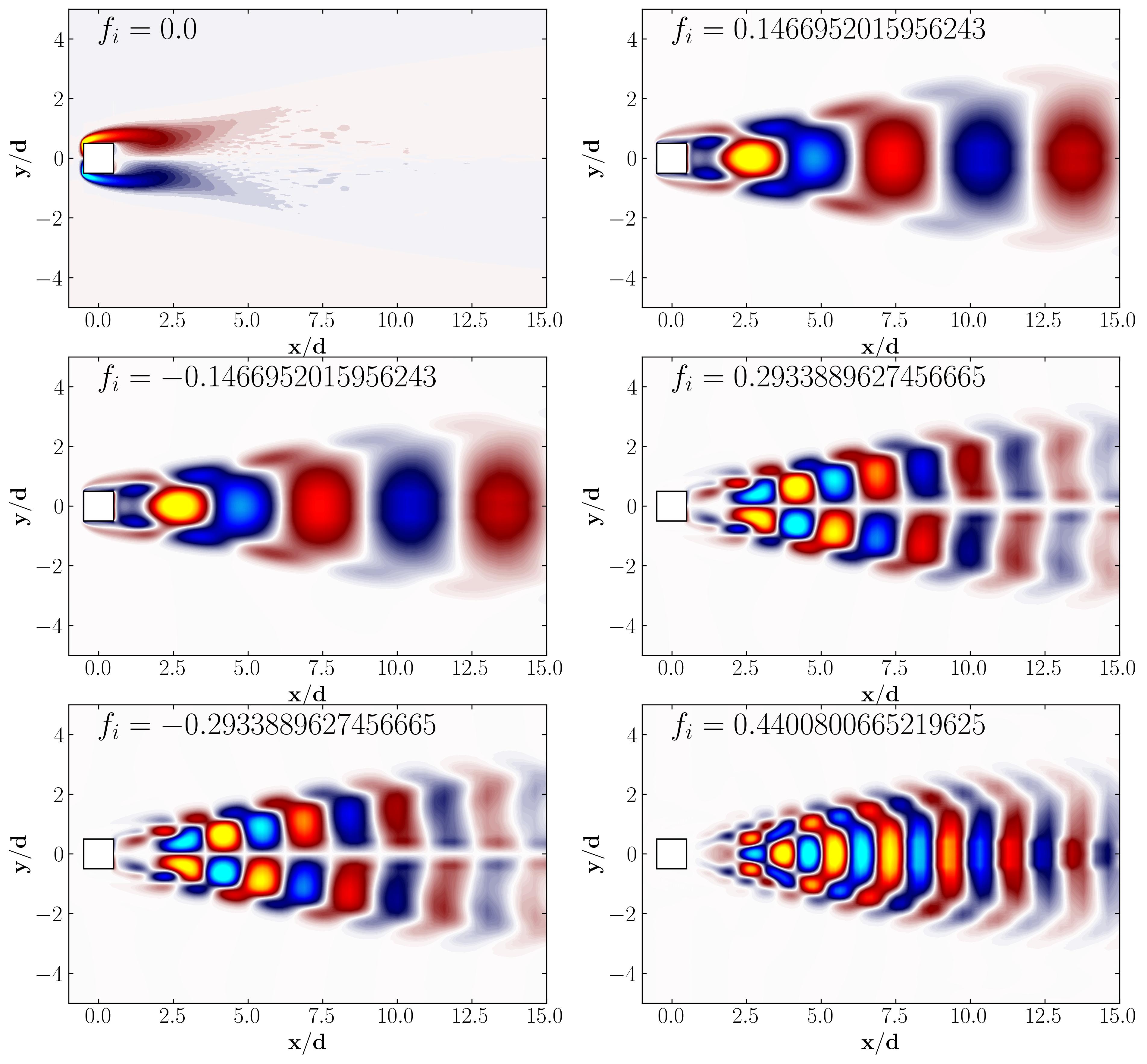
This visualization reveals the dominant spatial structures captured by each DMD mode. Each mode’s frequency helps distinguish between steady and oscillatory behaviors, uncovering flow characteristics at various scales.
Enjoy Reading This Article?
Here are some more articles you might like to read next: