In Computational Fluid Dynamics (CFD), understanding complex flow dynamics often requires the extraction of meaningful insights from vast simulation data. This blog dives into the essential process of gathering 3D snapshots from OpenFOAM simulations, a crucial step in enabling advanced modal decomposition techniques like SPOD and DMD. By streamlining data collection, we pave the way for uncovering the hidden structures and dynamics within turbulent flows.

Modern Computational Fluid Dynamics (CFD) simulations generate a wealth of data, offering a window into the intricate dynamics of fluid flows. However, unlocking actionable insights from this data requires more than visualization—it demands robust analytical techniques like modal decomposition. Whether it’s Dynamic Mode Decomposition (DMD), Spectral Proper Orthogonal Decomposition (SPOD), or other methods, the foundation for these techniques lies in assembling a well-structured dataset of time-varying snapshots.

In my previous article, I focused primarily on gathering 2D snapshots from simulations, as they are often sufficient for many analyses. However, certain scenarios demand more detailed insights, where the complexity of three-dimensional flow structures comes into play. In such cases, 3D snapshots become essential to capture the full intricacies of the simulated phenomena. In this blog, I focus on the process of gathering 3D snapshots from OpenFOAM simulations, a crucial step for preparing data suitable for modal decomposition. From configuring OpenFOAM to extract volumetric fields to organizing and post-processing the data, we’ll cover practical strategies to make this workflow efficient and accessible. By the end, you’ll have a clear roadmap to extract, organize, and analyze 3D flow data, unlocking its full potential for advanced analysis.

Lets Begin!!!

Example Case

To guide this tutorial on extracting 3D snapshots from a simulation, we will focus on the dynamics of three-dimensional flow around a square cylinder at a Reynolds number of 260. The flow will be simulated using Direct Numerical Simulations (DNS) implemented in OpenFOAM, following a setup closely aligned with the configuration outlined by Bai and Alam (2018) for reference.

The choice of this case is intentional. The wake generated behind the cylinder serves as a classic example of periodic (Kármán) vortex shedding—a phenomenon characterized by the alternating shedding of vortices, producing a periodic flow regime defined by a dominant frequency and its harmonics. At a Reynolds number of 260, the wake transitions into a fully three-dimensional structure, showcasing intricate vortex dynamics. These features make it an ideal candidate for this tutorial. Additionally, replicating a well-documented case allows us to effectively validate the simulated flow physics against published results. For guidance on setting up an unsteady case in OpenFOAM, refer to this article.

The key aspect of setting up a case for modal decomposition and collecting 3D snapshots lies in correctly configuring the system folder. This folder serves as the central hub for defining the numerical parameters of your simulation. Before initiating data collection, it is critical to ensure that the flow within the domain has reached a fully developed state. This involves allowing sufficient time for transient effects to subside, ensuring the flow attains stable and representative behavior.

A fully developed flow state is achieved when the flow characteristics stabilize and no longer exhibit significant variations over time or distance. For our case, which involves a quasi-periodic vortex shedding phenomenon, the goal is to reach a statistically stationary flow field. This requires running the simulation until random fluctuations diminish and the flow stabilizes. To achieve this, we will initially run the simulation for a duration equivalent to 20 Through Times. A Through Time represents the time it takes for a fluid particle to traverse the domain’s length undisturbed and is calculated as:

By running the simulation for this duration, we can capture a converged transient solution, setting the system/constant/endTime parameter appropriately.

To determine the time step, Δ𝑡, a Courant-Friedrichs-Lewy (CFL) number of ≤ 0.8 is used to ensure numerical stability. Given the minimum element size (Δ𝑥) and the free-stream velocity (𝑈_{ref}), the time step is calculated as:

This value is then assigned to the deltaT parameter in the controlDict file. By adhering to these criteria, we ensure that the time discretization is fine enough to accurately capture the flow dynamics while maintaining numerical stability.

Snapshot data extraction

Let’s dive into the data collection process, a critical step for performing modal decomposition analysis. Our goal is to capture multiple snapshots of the flow field, each corresponding to a distinct time instance. Following conventions in the literature, the number of snapshots is typically chosen as $2^n$ snapshots, where n depends on the specific case and user requirements. For this case, we will extract between 256 and 1024 snapshots. However, it’s essential to ensure that data collection begins only after the flow has reached a fully developed, statistically stable state. As such, snapshots will be gathered after the endTime specified in the simulation setup.

There are several methods to collect 3D volume snapshots from OpenFOAM simulations. In this tutorial, I will demonstrate one of the simplest approaches—using functionObjects. Specifically, we’ll use the vtkWrite function object to extract 3D volume fields from the simulation, as shown below:

  vtkWrite1
	{
		type            vtkWrite;
		libs            (utilityFunctionObjects);
		//timeStart		889.031;
		//timeEnd         1000;
		writeControl    timeStep;
		writeInterval   25;
		format          ascii;
		legacy          false;
		decompose       false;
		internal		true;
		boundary		false;
		interpolate true;
		fields          (U p);

		selection
		{
			box 
				{ 
					action  use; 
					source  box; 
					box     (-0.2 -0.5 -0.6) (2.4 0.5 0.6); 
				} 
		}
	}

This function object writes fields in VTK (XML or legacy) format, allowing for the export of cell-based or point-interpolated values for volume fields. Crucially, it enables the user to define a region of interest through the selection dictionary. But what exactly do we mean by the region of interest?

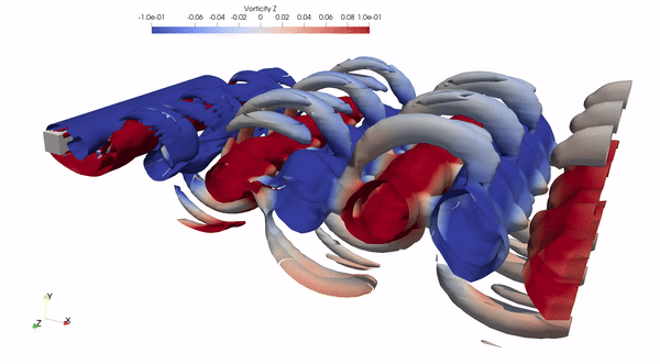
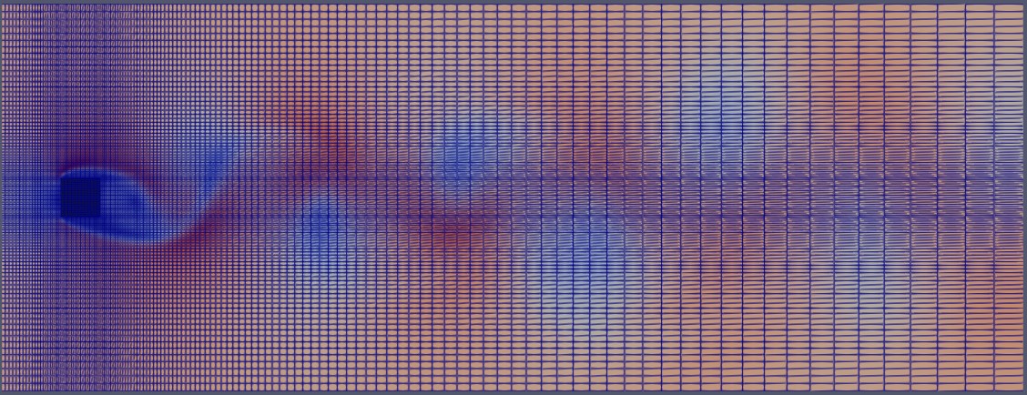
Below, we illustrate the full 3D domain of the simulated case—flow around a square cylinder at Re=260:

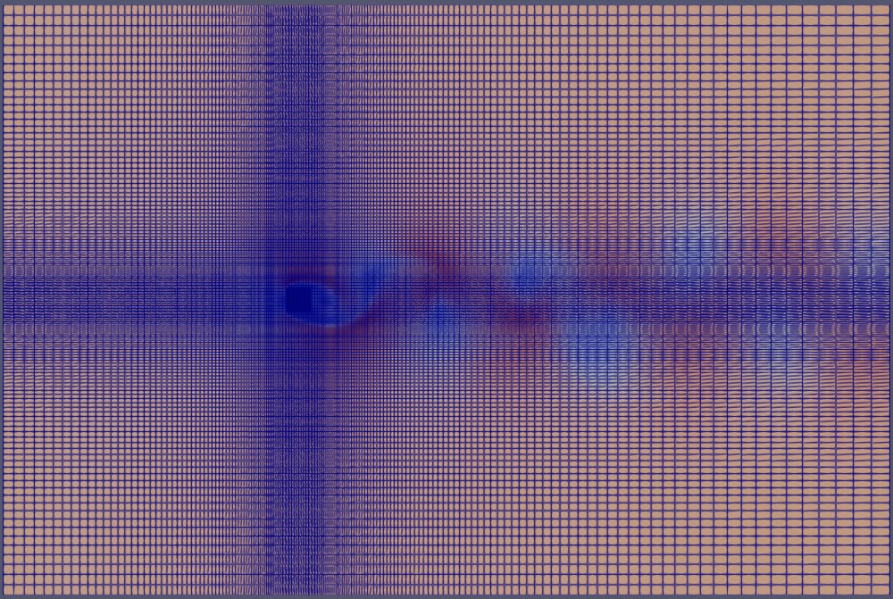
The meshing of this domain appears as follows:

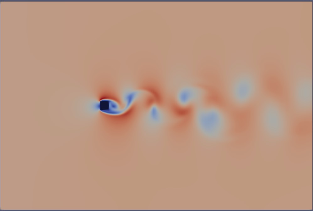
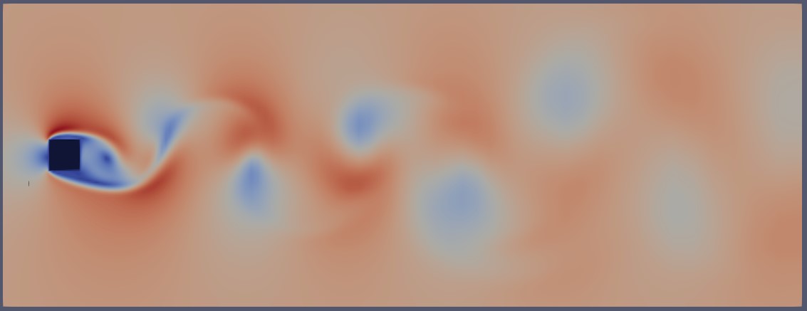
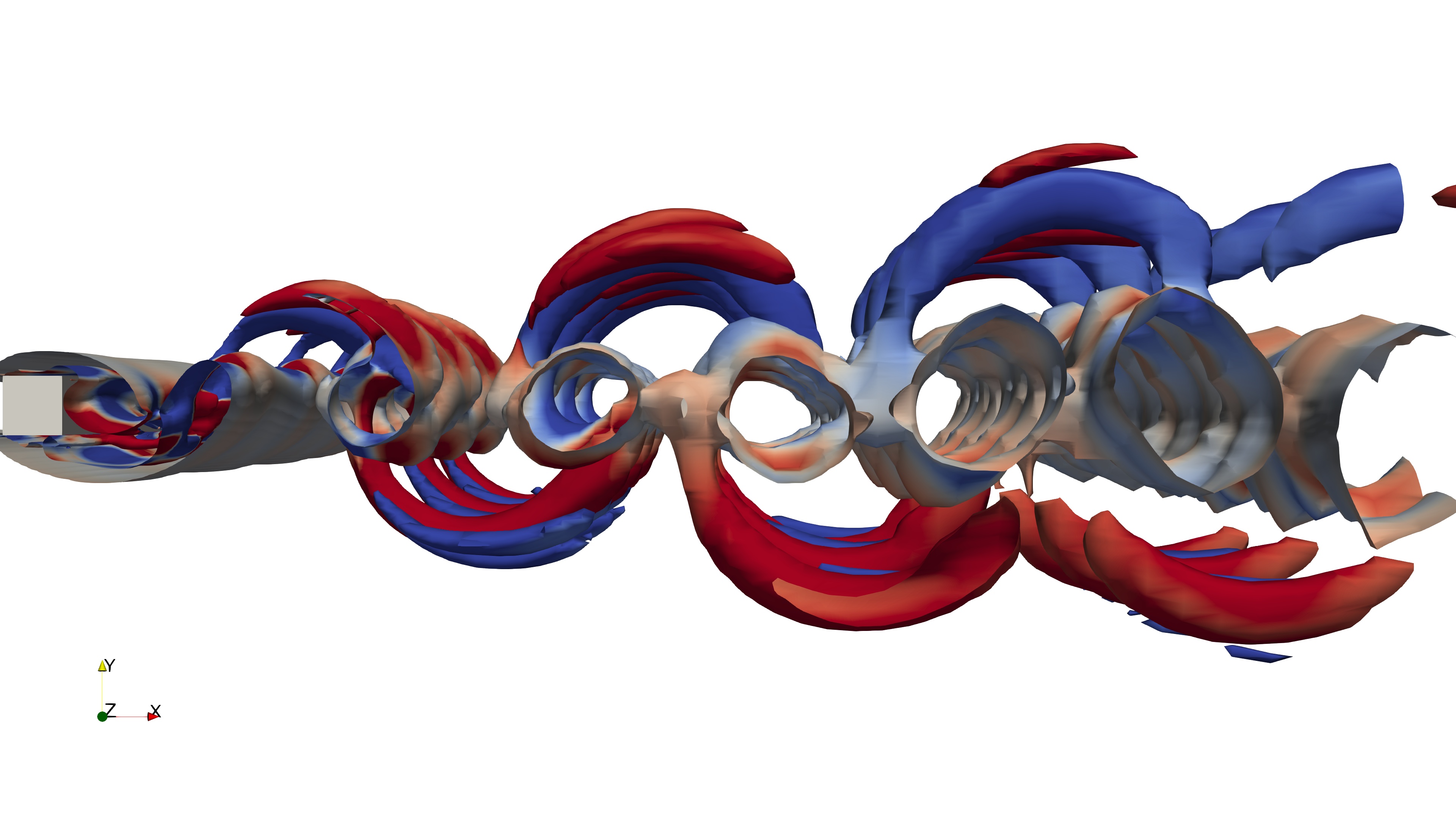
However, for our analysis, we are only interested in a specific region—a 3D box around the square cylinder, as shown below:

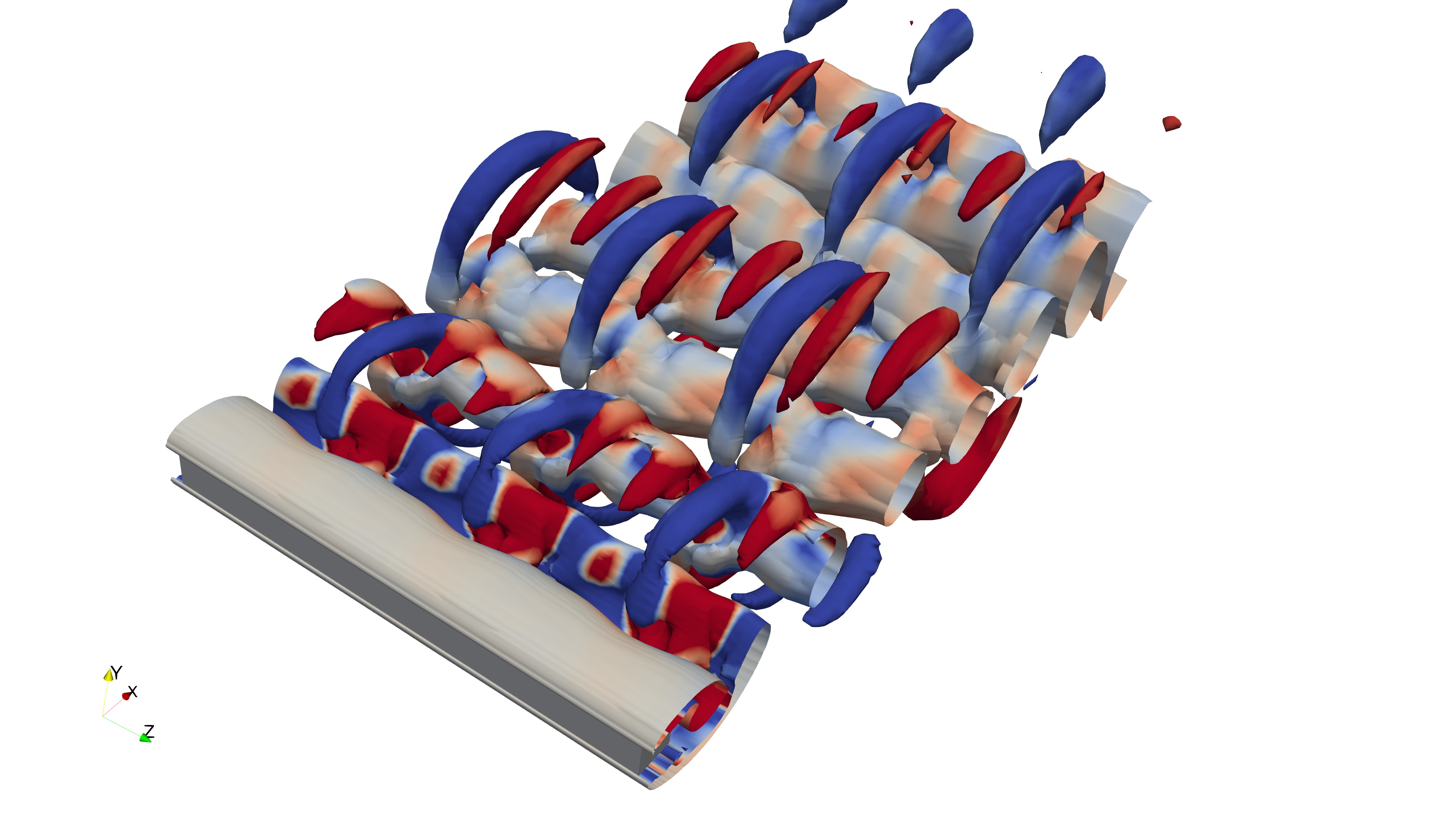
Here is the extracted mesh within the defined region of interest:

This region of interest is defined by a bounding box that spans the width and height of the wake. Essentially, we only need the volume fields and mesh information contained within this bounding box. In simpler terms, we aim to extract the 3D mesh region around the flow, as shown below:

To achieve this, we configure the selection dictionary as follows:

selection
{
	box 
		{ 
			action  use; 
			source  box; 
			box     (-0.2 -0.5 -0.6) (2.4 0.5 0.6); 
		} 
}

The vtkWrite function is primarily designed to extract cell-centered values of the volume field. However, for modal decomposition applications using Python, point-interpolated values are required. Additionally, we are only interested in the internal fields or volume fields, not the boundary fields. To optimize storage and focus exclusively on point-interpolated values, we will configure the vtkWrite function object with the following settings:

internal		true;
boundary		false;
interpolate true;

Next, I will run the simulation again, starting from the fully developed state and extracting the region defined by the selection dictionary every 25 writeInterval steps. This approach will allow me to collect approximately 250 snapshots. Keep an eye out for the following output during the simulation:

vtkWrite1 output Time: 1996.8
    Internal  : "postProcessing/vtkWrite1/3D_Bai_00037401/internal.vtu"
    volScalarField(p)
    volVectorField(U)
    volScalarField->point(p)
    volVectorField->point(U)

These snapshots will be stored in the postProcessing folder of your case directory as shown below:

vtkWrite1
├── 3D_Bai.vtm.series
├── 3D_Bai_00037401
│   └── internal.vtu
└── 3D_Bai_00037401.vtm

In this structure, the internal.vtu file contains the 3D snapshot data.

Construction snapshot matrix

Now, let’s assume you’ve run the simulation and collected at least 250 3D snapshots, all stored in internal.vtu files, structured as shown earlier. We will now use Python to construct the snapshot matrix, which will later be used for modal decomposition analysis. To get started, open a Jupyter notebook and import the necessary modules:

import matplotlib.colors
import matplotlib.pyplot as plt
import numpy as np
import pandas as pd
import fluidfoam as fl ### Most Important
import scipy as sp
from matplotlib.colors import ListedColormap
import os
import io
import pyvista as pv
%matplotlib inline
plt.rcParams.update({'font.size' : 18, 'font.family' : 'Times New Roman', "text.usetex": True})

Next, assign the appropriate path variables and define the location of each snapshot file. At this point, the internal.vtu file is stored within a subdirectory named 3D_Bai_00037401.

# Path variables
Path = 'E:/Blog_Posts/Simulations/3D_Bai/'
Surfaces = 'E:/Blog_Posts/Simulations/3D_Bai/postProcessing/vtkWrite1/'

# File variables
Files = os.listdir(Surfaces)

Next, I will use PyVista to read the internal.vtu file and estimate its size:

Data = pv.read(Surfaces + Files[0] + '/internal.vtu')
grid = Data.points
x = grid[:,0]
y = grid[:,1]
z = grid[:,2]
rows, columns = np.shape(grid)
print('rows = ', rows, ', columns = ', columns)

#### Output
#### rows =  624537 , columns =  3

This output indicates that the extracted VTK file contains data at 624,537 points, and each point is represented in a 3D space (x, y, z).

Next, let’s read the point arrays contained within this file:

print(Data.array_names)

#### Output
#### ['TimeValue', 'p', 'U', 'p', 'U']

Next, we will use a for loop to construct the snapshot matrix. Note that this step can be time-consuming since we are reading 3D VTK files and arranging the data into a tall, thin matrix. As for the data to collect, one can choose either velocity or pressure; however, I opt to use the vorticity matrix for data analysis.

Data = pv.read(Surfaces + Files[0] + '/internal.vtu')
grid = Data.points
x = grid[:,0]
y = grid[:,1]
z = grid[:,2]
rows, columns = np.shape(grid)
print('rows = ', rows, 'columns = ', columns)

### For U
Snaps = len(Files)
data_Vort = np.zeros((rows,Snaps-1))
for i in np.arange(0,Snaps-1):
    data = pv.read(Surfaces + Files[i] + '/internal.vtu')
    gradData = data.compute_derivative('U', vorticity=True)
    grad_pyvis = gradData.point_data['vorticity']
    data_Vort[:,i:i+1] = np.reshape(grad_pyvis[:,2], (rows,1), order='F')

np.save(Path + 'VortZ.npy', data_Vort)

This matrix, data_Vort, will be used for modal decomposition analysis going forward. Given that we know the size of the file and the shape of the initial data, it will be easy to reconstruct a single data instance using PyVista.

In this blog, we’ve walked through the process of extracting 3D snapshots from OpenFOAM simulations and preparing the data for modal decomposition analysis. By leveraging tools like PyVista and carefully configuring function objects, we’ve been able to capture, process, and organize the data into a snapshot matrix ready for further analysis. The approach we’ve discussed not only facilitates efficient data collection but also ensures that the information is structured in a way that is suitable for more advanced techniques like modal decomposition. As we move forward with modal decomposition and other data-driven analyses, the ability to extract and organize high-dimensional flow data will become increasingly important in gaining deeper insights into complex fluid dynamics. In my next article, I will focus on other methods of collecting snapshot data using OpenFOAM.