3D POD and Visualization with OpenFOAM and Python
In fluid dynamics, understanding the intricate patterns hidden within three-dimensional flow data is crucial for advancing both research and engineering applications. Proper Orthogonal Decomposition (POD) serves as a powerful tool to extract dominant flow structures, simplifying complex dynamics into comprehensible insights. This article takes you through the step-by-step application of three-dimensional POD using OpenFOAM simulation data and Python wizardry, emphasizing visualization for enhanced interpretation. Whether you’re a CFD enthusiast or a seasoned researcher, this guide will equip you with practical skills to explore and analyze multi-dimensional fluid flows effectively.
Understanding the spatio-temporal dynamics of fluid flow is a cornerstone of Computational Fluid Dynamics (CFD) analysis. Proper Orthogonal Decomposition (POD) is a widely-used technique for uncovering dominant flow structures in complex datasets, offering a gateway to simplifying and interpreting intricate flow dynamics. In this blog, we dive into the application of 3D POD using OpenFOAM simulation data, processed using Python and visualized with ParaView. By transforming CFD results into insightful visual patterns, this approach enhances our ability to analyze and comprehend multi-dimensional fluid behavior.
This article builds upon the methodology discussed in my previous blog - Extracting 3D Snapshots from OpenFOAM for Modal Decomposition Analysis. There, we explored how to gather and preprocess simulation snapshots, a critical first step for modal analysis techniques like POD. Now, we take the next leap, leveraging those extracted snapshots to perform a full 3D POD analysis and create visualizations that bring flow structures to life. If you’ve followed the steps outlined earlier, you’re well-prepared to embark on this deeper dive into flow decomposition and visualization.
If you’re new to modal decomposition or OpenFOAM, I recommend checking out my previous articles, which provide a solid foundation in the POD methodology and its underlying mathematical principles.
In this tutorial, we’ll once again explore the dynamics of three-dimensional flow around a square cylinder at a Reynolds number of 260. For your convenience, a reference case setup is available here.
Lets Begin!!!
3D Proper Orthogonal Decomposition
In my previous article, we explored the process of extracting 3D snapshots from OpenFOAM simulations and preparing the data for modal decomposition analysis. As part of that workflow, we assembled a matrix, data_Vort, which will serve as the foundation for our POD analysis in this tutorial. Now, let’s dive back in by opening a Jupyter Notebook and importing the necessary modules.
import matplotlib.colors
import matplotlib.pyplot as plt
import numpy as np
import pandas as pd
import fluidfoam as fl ### Most Important
import scipy as sp
from matplotlib.colors import ListedColormap
import os
import io
import pyvista as pv
%matplotlib inline
plt.rcParams.update({'font.size' : 18, 'font.family' : 'Times New Roman', "text.usetex": True})
Next, we’ll assign the necessary path variables and define the data matrix:
# Path variables
Path = 'E:/Blog_Posts/Simulations/3D_Bai/'

# Constants
d = 0.1
Ub = 0.039
At this stage, we’ll import the data_Vort matrix and verify its shape:
# Import matrix
data_Vort = np.load(Path + 'VortZ.npy')

# Check matrix shape
data_Vort.shape
### OUTPUT
### (624537, 161)
The matrix shape reveals the spatial and temporal degrees of freedom in our dataset. Here, the 3D mesh consists of 624,537 elements with 161 time-varying snapshots for analysis. Understanding the structure of your dataset is crucial for ensuring accurate and efficient modal decomposition!
For this tutorial, I will use MODULO, a cutting-edge software developed at the von Karman Institute for performing advanced data-driven decompositions. While initially designed for Multiscale Proper Orthogonal Decomposition (mPOD), MODULO has evolved to support a wide array of methods, including POD, SPOD, DFT, DMD, and more. Its standout feature is its efficiency: it processes large datasets by dividing them into manageable chunks, making it perfect for high-complexity applications. Furthermore, MODULO excels at handling non-uniform meshes through its weighted inner product approach, ensuring precise results.
If you’d like to learn more about MODULO, check out my earlier article here.
Let’s now import the MODULO package into our notebook:
from modulo_vki import ModuloVKI
Next, let’s initialize MODULO:
# Initialize MODULO object
m = ModuloVKI(data=np.nan_to_num(data_Vort), n_Modes=50)
This initialization configures the data_Vort matrix to be read into the MODULO POD class, specifying that the first 50 modes will be extracted from the dataset. Using MODULO, we’ll now compute POD with the Singular Value Decomposition (SVD) method, which is particularly well-suited for smaller datasets due to its generality and efficiency.
# POD via svd
Phi_P, Psi_P, Sigma_P = m.compute_POD_svd()

# Check matrix shapes
Phi_P.shape, Psi_P.shape, Sigma_P.shape
### OUTPUT
### ((624537, 50), (161, 50), (50,))
With POD successfully performed, we can now visualize the energy content of each POD mode along with the cumulative energy to gain insights into how energy is distributed across the modes.
Energy = np.zeros((len(Sigma_P),1))
for i in np.arange(0,len(Sigma_P)):
    Energy[i] = Sigma_P[i]/np.sum(Sigma_P)

X_Axis = np.arange(Energy.shape[0])
heights = Energy[:,0]

fig, axes = plt.subplots(1, 2, figsize = (12,4))
ax = axes[0]
ax.plot(Energy, marker = 'o', markerfacecolor = 'none', markeredgecolor = 'k', ls='-', color = 'k')
ax.set_xlabel('Modes')
ax.set_ylabel('Energy Content')

ax = axes[1]
cumulative = np.cumsum(Sigma_P)/np.sum(Sigma_P)
ax.plot(cumulative, marker = 'o', markerfacecolor = 'none', markeredgecolor = 'k', ls='-', color = 'k')
ax.set_xlabel('Modes')
ax.set_ylabel('Cumulative Energy')

plt.show()
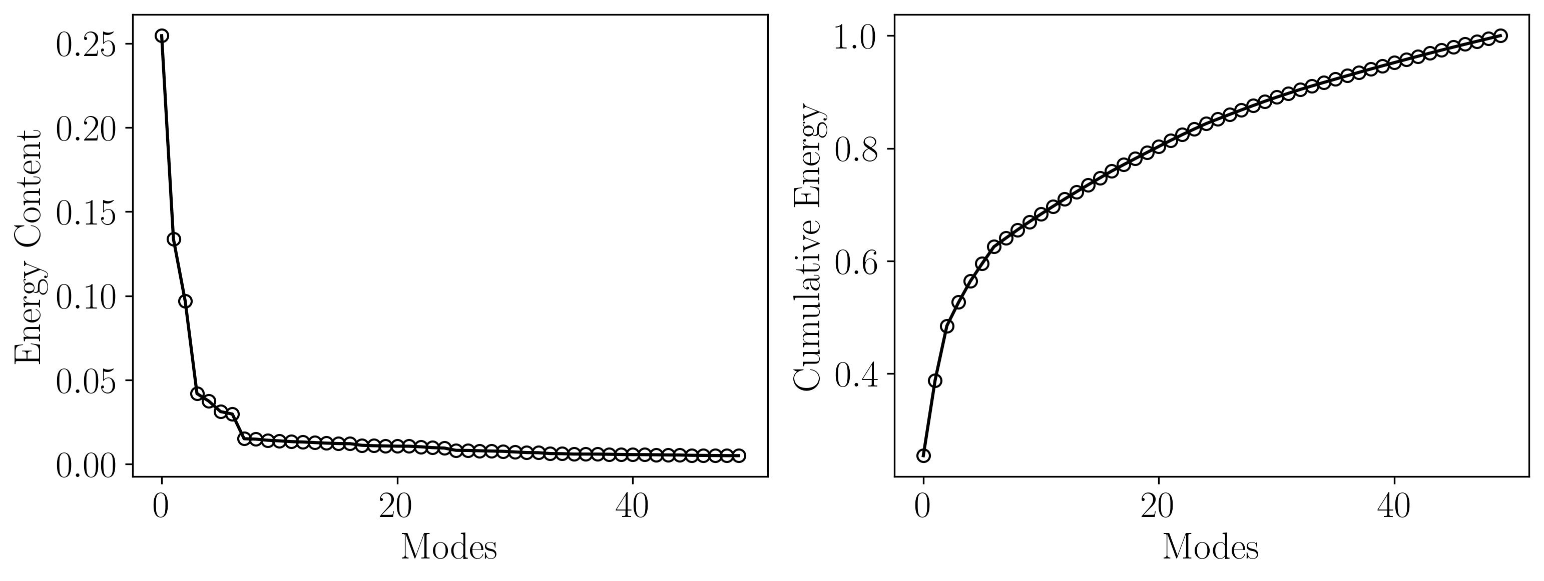
This plot illustrates that the first 10 POD modes capture approximately 67% of the total energy, indicating that a significant portion of the flow dynamics can be effectively represented with these modes. By focusing on these dominant modes, we achieve a substantial reduction in the dimensionality of the dataset, which simplifies further analysis and computational modeling. Such dimensionality reduction is especially valuable in scenarios where computational resources are limited or when developing reduced-order models (ROMs) for real-time simulations or control systems. Moreover, these modes often correspond to the most physically meaningful flow structures, allowing researchers to gain deeper insights into the underlying dynamics without being overwhelmed by less significant variations. This balance between accuracy and efficiency makes POD a powerful tool for analyzing complex fluid flows.
3D POD Visualization
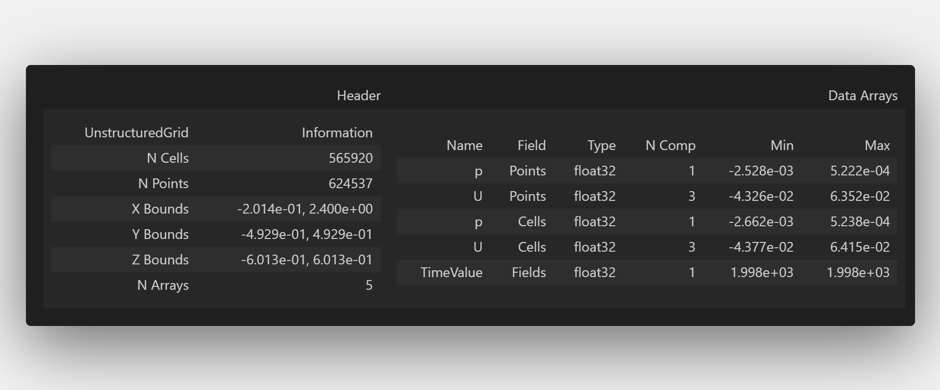
To visualize the POD output in 3D, we’ll use a combination of Python and ParaView. Python will be utilized to write the first 10 POD modes into a VTK file, which can then be opened in ParaView for detailed visualization. As a first step, we’ll read in the first snapshot from the simulation to serve as the base VTK file into which our output will be written:
# File location to write a VTK File
WhereWrite = 'E:/Blog_Posts/Simulations/3D_Bai/postProcessing/'

# First snapshot, base file
WriteFile = pv.read(Surfaces + Files[0] + '/internal.vtu')

WriteFile
Next, we’ll proceed to write the first 10 POD modes into this file for visualization.
Mode0 = Phi_P[:,0]*(d/Ub)
Mode1 = Phi_P[:,1]*(d/Ub)
Mode2 = Phi_P[:,2]*(d/Ub)
Mode3 = Phi_P[:,3]*(d/Ub)
Mode4 = Phi_P[:,4]*(d/Ub)
Mode5 = Phi_P[:,5]*(d/Ub)
Mode6 = Phi_P[:,6]*(d/Ub)
Mode7 = Phi_P[:,7]*(d/Ub)
Mode8 = Phi_P[:,8]*(d/Ub)
Mode9 = Phi_P[:,9]*(d/Ub)
Mode10 = Phi_P[:,10]*(d/Ub)

WriteFile.point_data['Mode0'] = Mode0
WriteFile.point_data['Mode1'] = Mode1
WriteFile.point_data['Mode2'] = Mode2
WriteFile.point_data['Mode3'] = Mode3
WriteFile.point_data['Mode4'] = Mode4
WriteFile.point_data['Mode5'] = Mode5
WriteFile.point_data['Mode6'] = Mode6
WriteFile.point_data['Mode7'] = Mode7
WriteFile.point_data['Mode8'] = Mode8
WriteFile.point_data['Mode9'] = Mode9
WriteFile.point_data['Mode10'] = Mode10

WriteFile.save(WhereWrite + 'Visualize_Final.vtu')

WriteFile
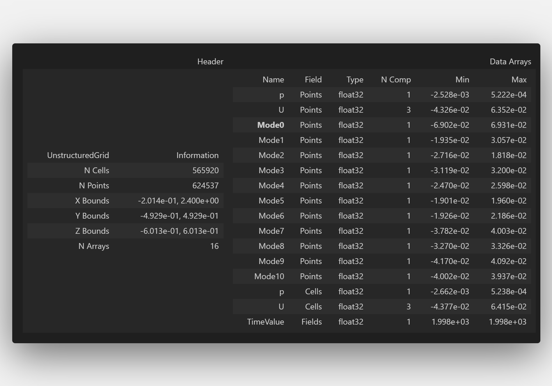
PS: Don’t worry about the .vtu extension—it’s simply a VTK file!
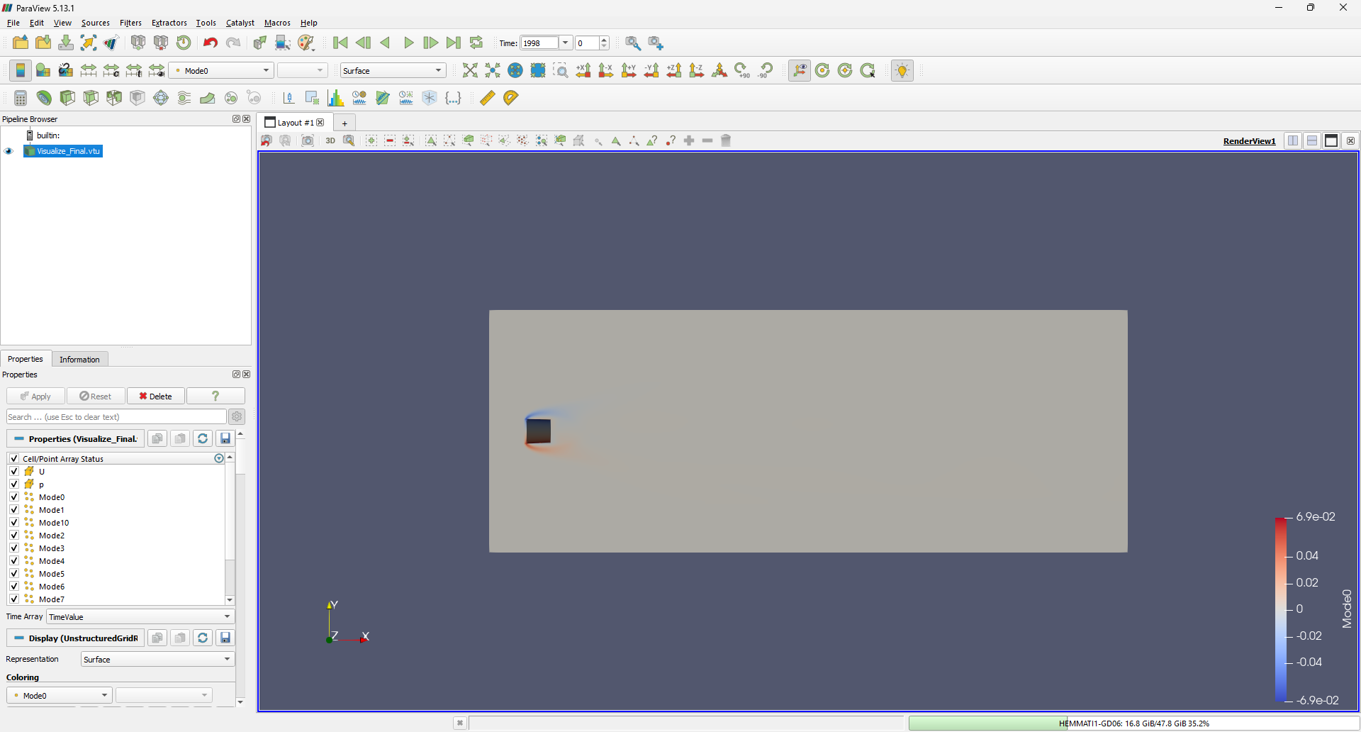
Now, let’s open this VTK file in ParaView. Once loaded, it should look something like this:
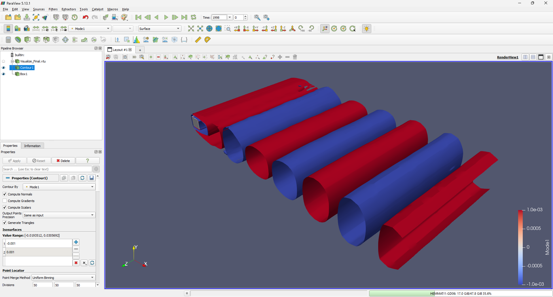
To visualize the modes, navigate to Filters -> Common -> Contour. Specify the appropriate ranges for the iso-surfaces and add a square cylinder representation by selecting Sources -> Geometric Shapes -> Box. The first mode should appear as follows:
Similarly, you can visualize the first six modes:
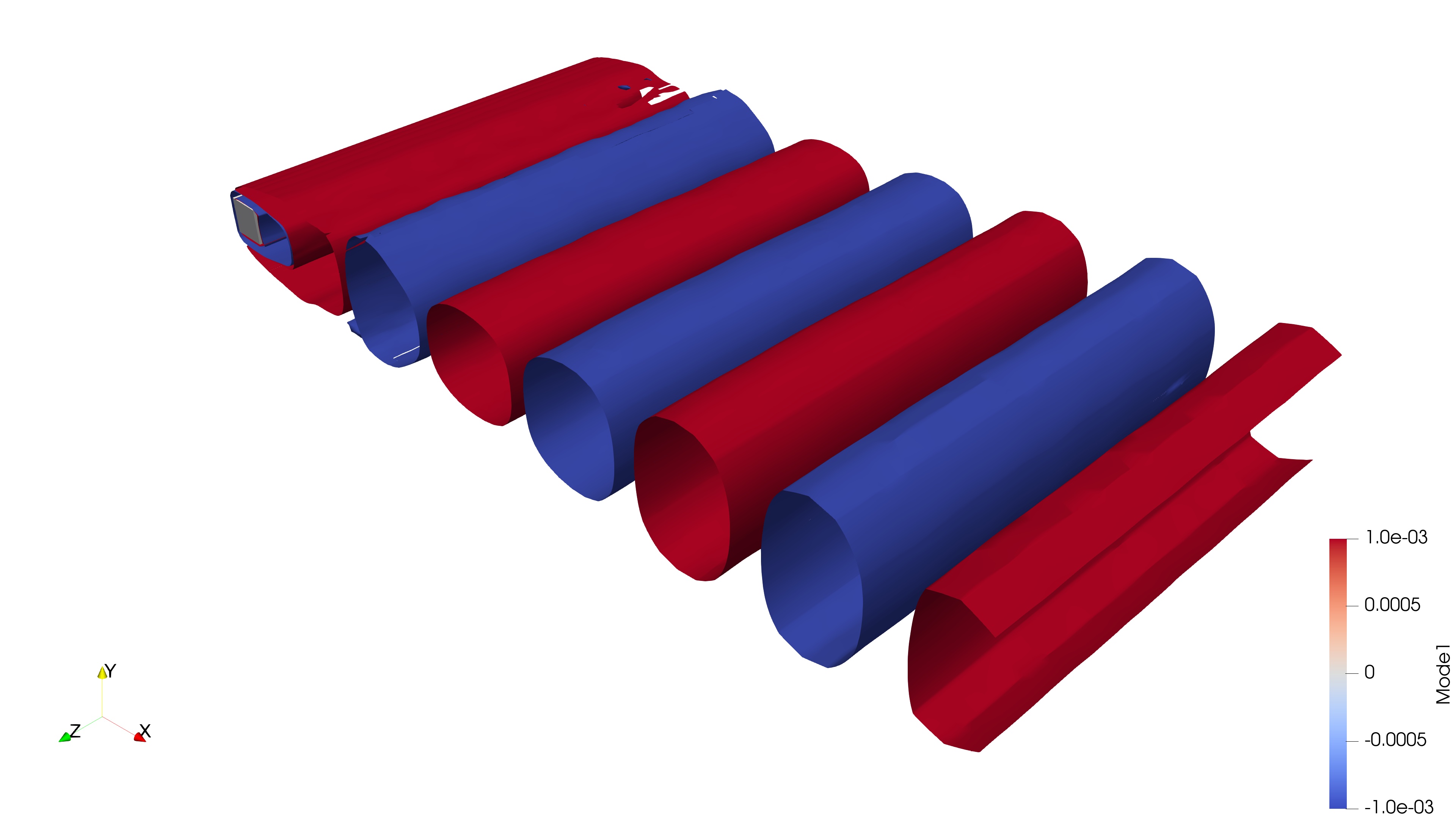
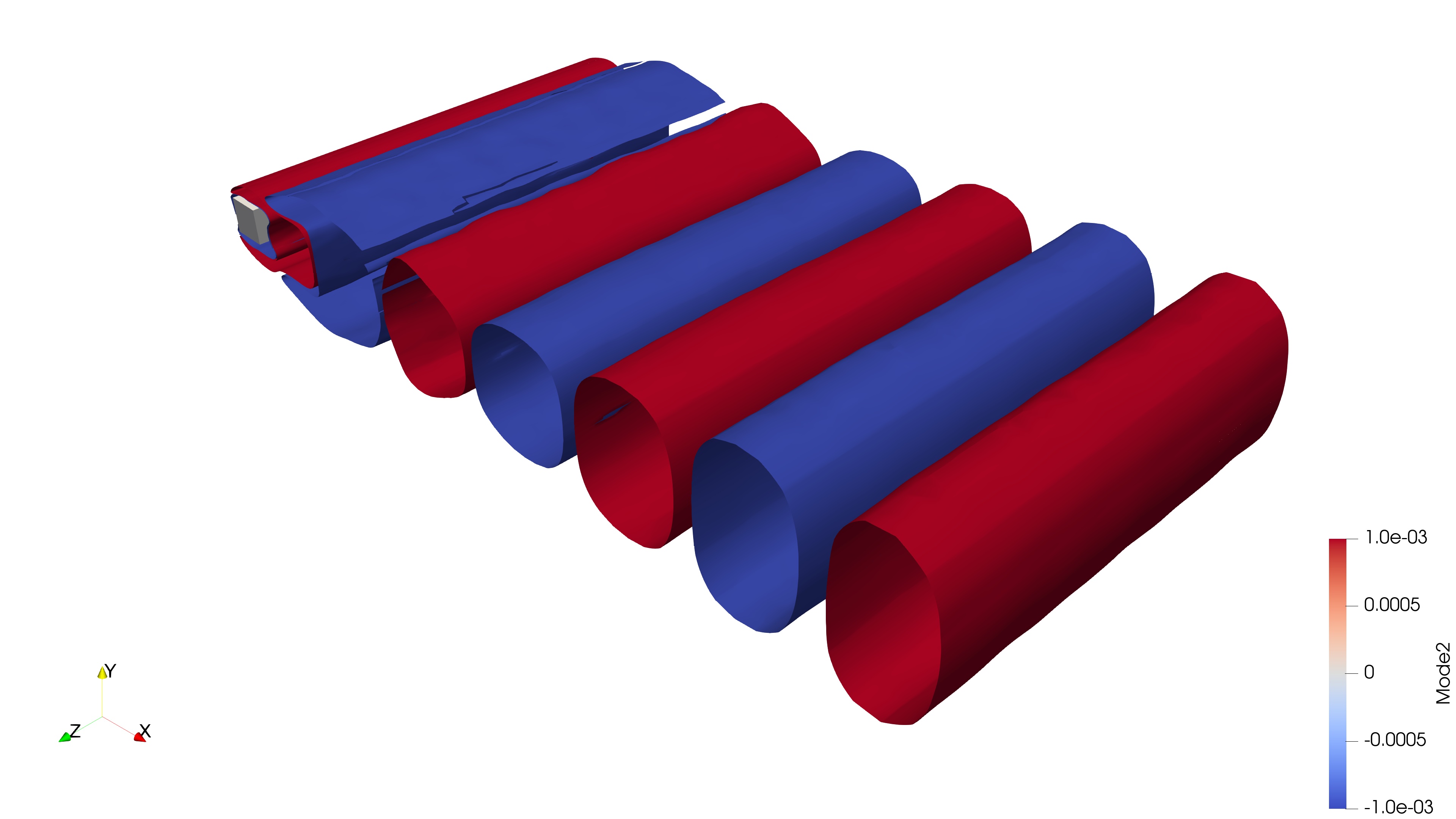
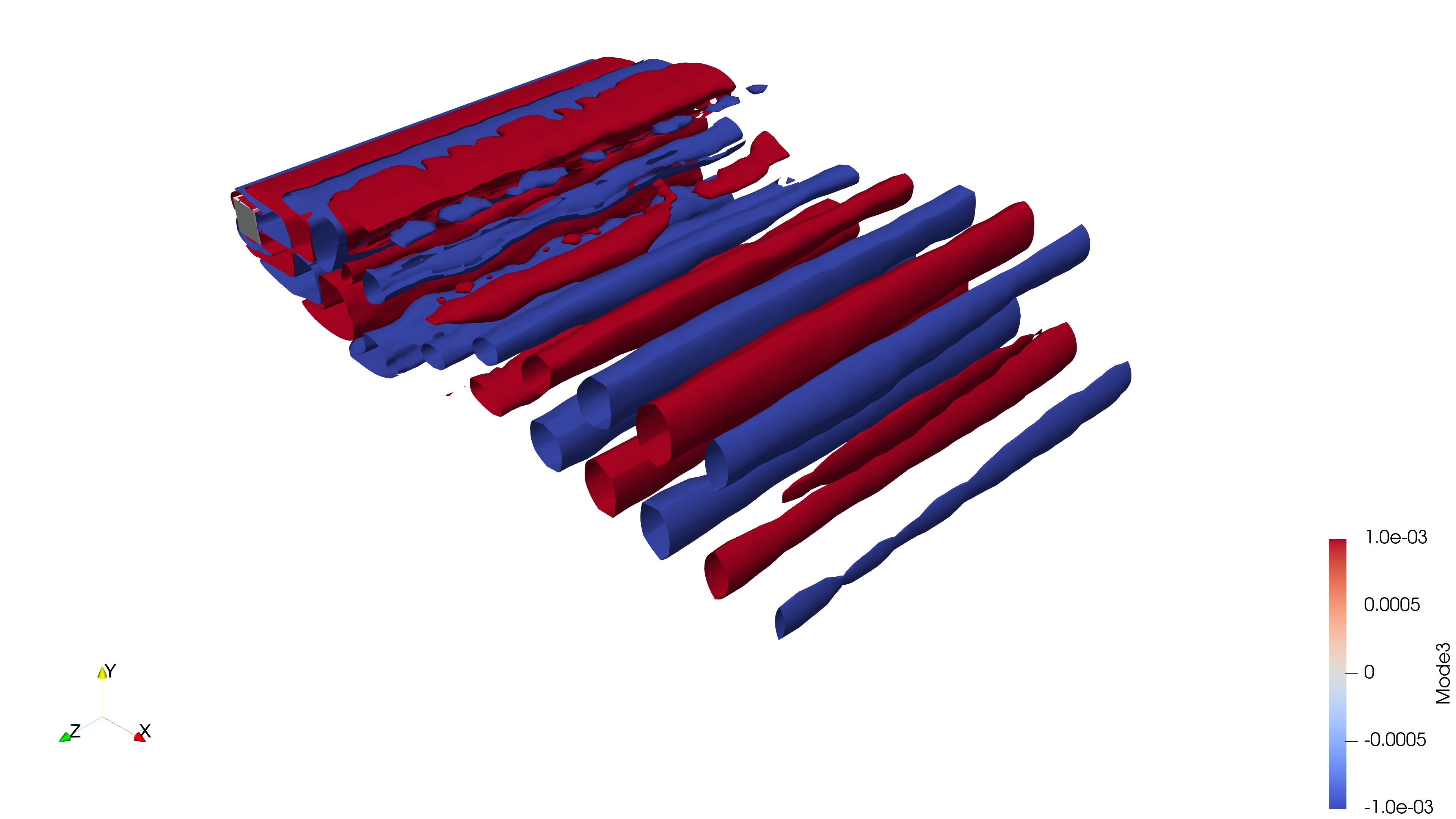
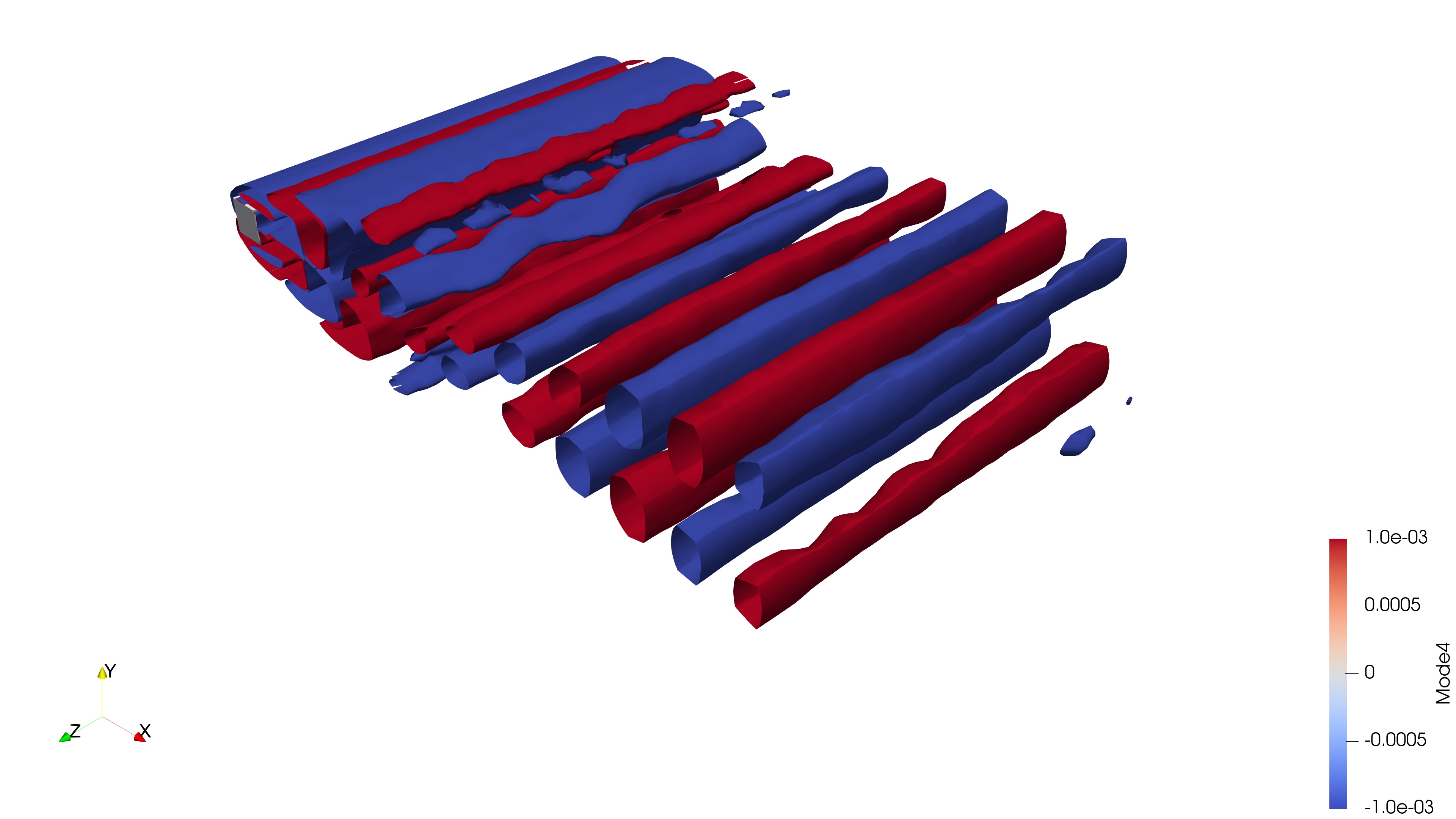
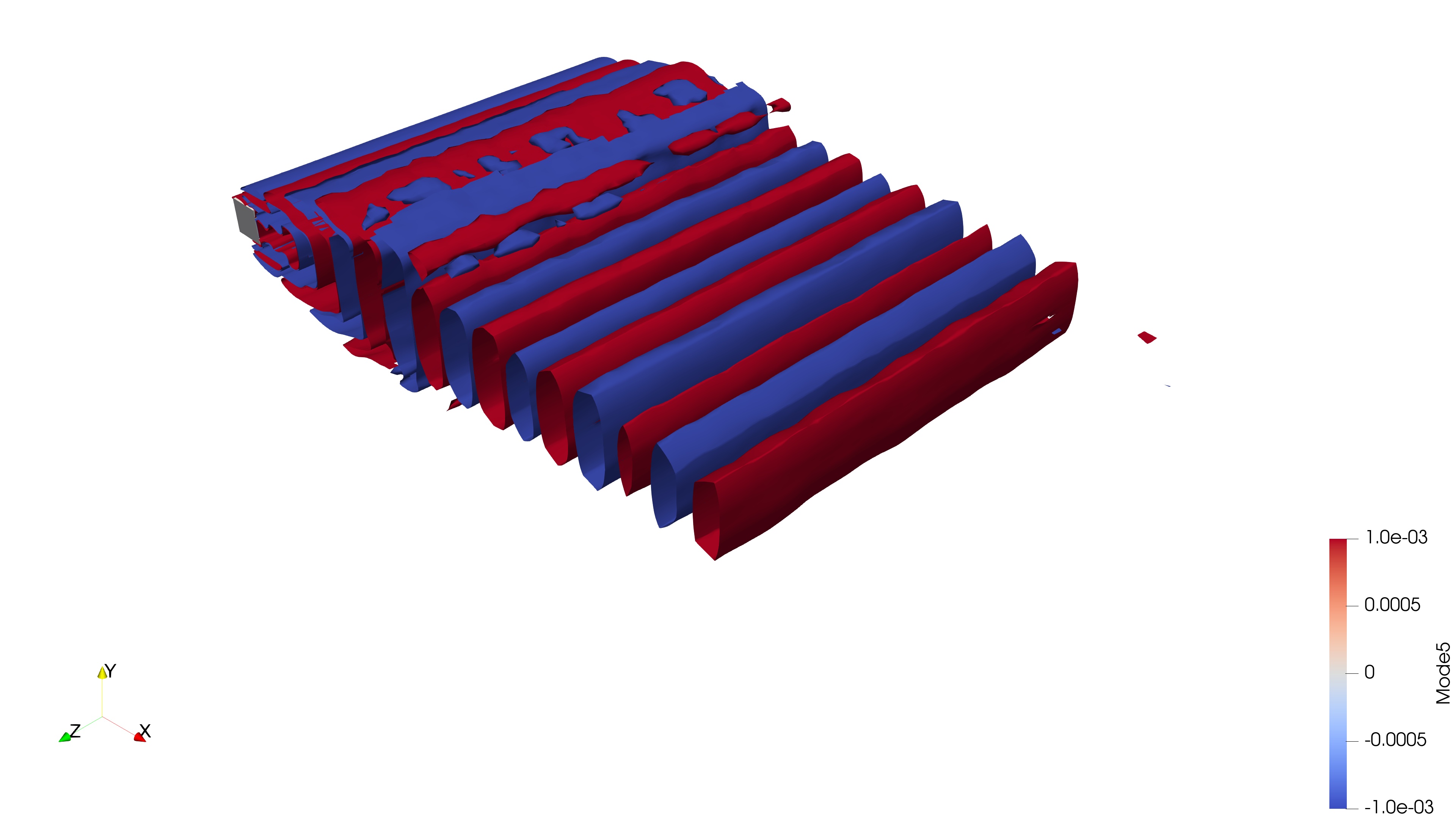

3D visualization provides valuable insights into the spanwise vortex activity within the system. Exploring these 3D instabilities and understanding the three-dimensionality of the flow is crucial for characterizing the dynamics of this configuration.
Next, we’ll take a 2D slice of the data to analyze in Python. While ParaView is excellent for visualizing flow structures, Python offers greater control over the output, making it ideal for detailed analysis. To create a slice, use Filters -> Common -> Slice and define a 2D slice along the Z-direction:
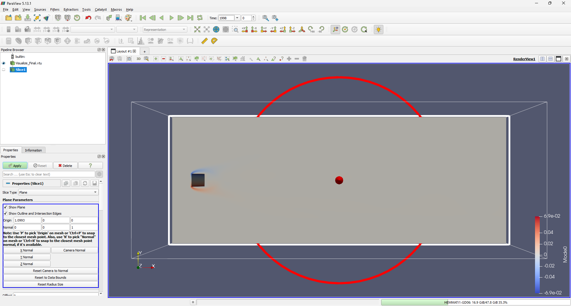
Once the slice is created, save it by selecting File -> Save Data and choosing VTK PolyData File (*.vtp) as the file format.
Finally, we’ll read this slice back into our Jupyter Notebook and extract the modes for further analysis:
# Read 2D slice
Data2D = pv.read(WhereWrite + 'Slice1.vtp')
grid = Data2D.points
x = grid[:,0]
y = grid[:,1]
z = grid[:,2]
rows, columns = np.shape(grid)

# Extract Modes
Mode1 = Data2D.point_data['Mode1']
Mode2 = Data2D.point_data['Mode2']
Mode3 = Data2D.point_data['Mode3']
Mode4 = Data2D.point_data['Mode4']
Mode5 = Data2D.point_data['Mode5']
Mode6 = Data2D.point_data['Mode6']
Now, using simple Python plotting routines, we can visualize the first six modes on this 2D slice:
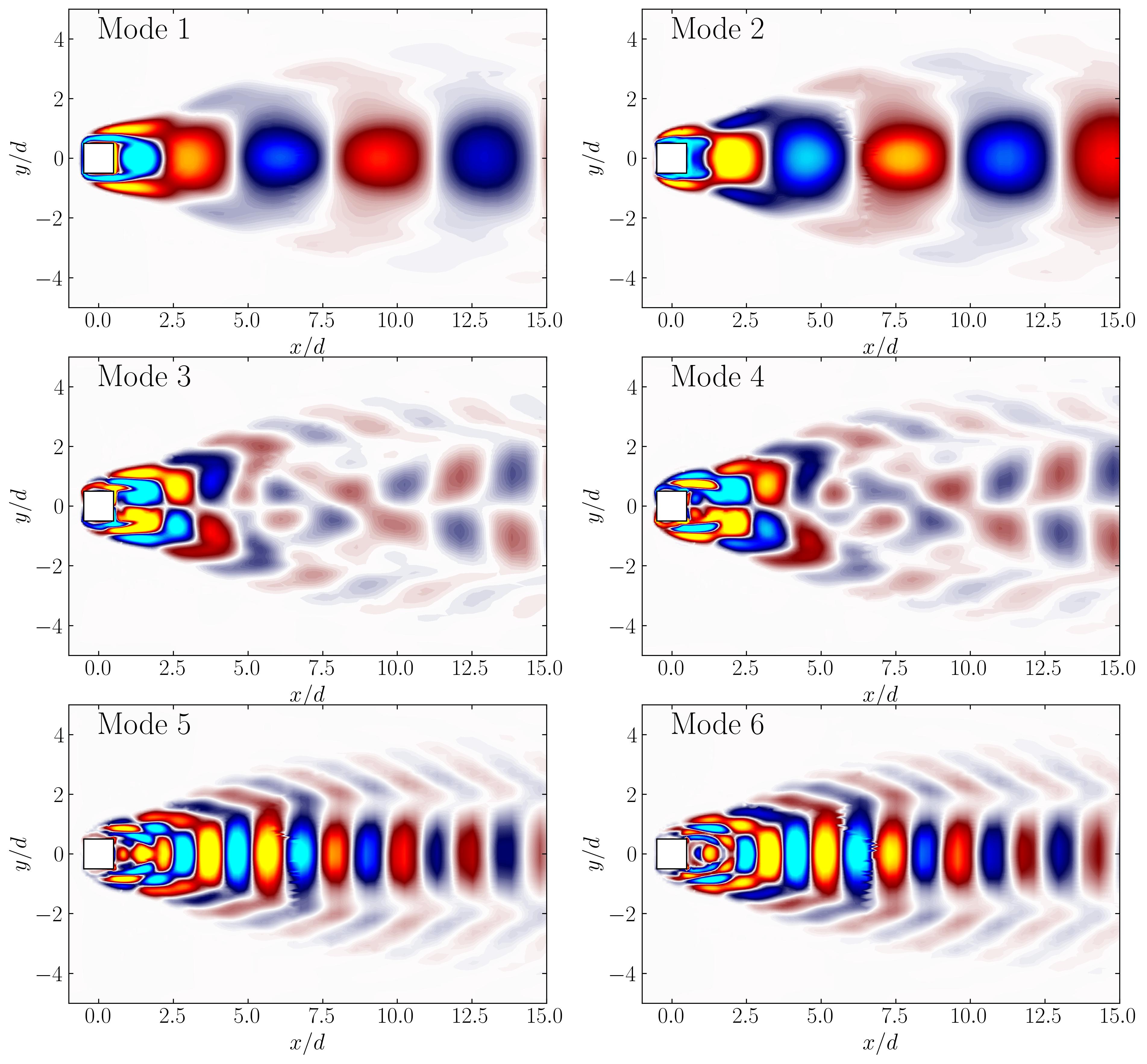
In this tutorial, we explored how to apply Proper Orthogonal Decomposition (POD) to analyze 3D fluid flow data from OpenFOAM simulations. By leveraging MODULO for efficient mode extraction and Python for visualization, we were able to gain valuable insights into the flow’s dominant structures and energy distribution. We also demonstrated how to visualize these modes in both 3D using ParaView and in 2D slices for more detailed analysis. The combination of these tools provides a powerful approach for investigating complex flow phenomena, offering both clarity and computational efficiency.
Enjoy Reading This Article?
Here are some more articles you might like to read next: