Understanding the complex, dynamic behavior of fluid flows often requires more than just time-averaged statistics. Dynamic Mode Decomposition (DMD) offers a powerful, data-driven approach to uncover the temporal evolution of coherent structures within CFD datasets. In this blog, we’ll dive into the process of applying DMD to three-dimensional flow fields simulated using OpenFOAM and visualize the resulting modes with Python and ParaView. By combining these tools, we can unravel the intricate interactions that define unsteady flows, providing insights into both dominant patterns and transient dynamics.

Understanding the complex dynamics of unsteady fluid flows requires tools that go beyond traditional averaging techniques. In my previous article on 3D Proper Orthogonal Decomposition (POD), we explored how to identify the dominant spatial structures in a flow field using OpenFOAM data. While POD is invaluable for spatial decomposition, it lacks the ability to capture temporal evolution—a crucial aspect when studying unsteady or transient phenomena.

This is where Dynamic Mode Decomposition (DMD) shines. DMD bridges the gap by uncovering modes that represent both spatial patterns and their associated temporal behavior. In this blog, we’ll build on the groundwork laid in my 3D POD article and demonstrate how to apply DMD to three-dimensional flow data. Using OpenFOAM for simulations, Python for data handling, and ParaView for visualization, we’ll uncover the temporal dynamics of a classic fluid flow problem. By the end of this tutorial, you’ll see how DMD complements POD, enabling a deeper understanding of unsteady flows.

In this tutorial, I’ll once again explore the dynamics of three-dimensional flow around a square cylinder at a Reynolds number of 260. For your convenience, a reference case setup is available here.

Lets Begin!!

3D Dynamic Mode Decomposition

Building on the foundations from the previous article, we’ll use the pre-assembled snapshot matrix, data_Vort, along with the MODULO package to perform 3D Dynamic Mode Decomposition (DMD). This step-by-step guide will demonstrate how to set up the necessary environment, process the data, and extract meaningful temporal dynamics.

We’ll start by loading the required Python modules and defining the necessary path variables in a Jupyter Notebook:

import matplotlib.colors
import matplotlib.pyplot as plt
import numpy as np
import pandas as pd
import fluidfoam as fl ### Most Important
import scipy as sp
from matplotlib.colors import ListedColormap
import os
import io
import pyvista as pv
%matplotlib inline
plt.rcParams.update({'font.size' : 18, 'font.family' : 'Times New Roman', "text.usetex": True})

# Path variables
Path = 'E:/Blog_Posts/Simulations/3D_Bai/'

# Constants
d = 0.1
Ub = 0.039

Next, import the data_Vort matrix, which contains the 3D snapshots of the vorticity field, and check its dimensions:

# Import matrix
data_Vort = np.load(Path + 'VortZ.npy')

# Check matrix shape
data_Vort.shape
### OUTPUT
### (624537, 161)

This output confirms that the dataset consists of a 3D spatial mesh with 624,537 elements and 161 temporal snapshots.

To proceed with the DMD analysis, we’ll initialize the MODULO package:

from modulo_vki import ModuloVKI

# Initialize MODULO object
m = ModuloVKI(data=np.nan_to_num(data_Vort), n_Modes=150)

DMD requires the sampling frequency of the dataset, which corresponds to the time interval between consecutive snapshots in the simulation. Retrieve this information from the OpenFOAM simulation setup:

# Sampling time and frequency
dt = 0.05*25
F_S = 1/dt

Finally, compute the DMD modes, eigenvalues, frequencies, and initial amplitudes using the MODULO package:

# Compute DMD using MODULO
Phi_D, Lambda, freqs, a0s = m.compute_DMD_PIP(False, F_S=F_S)

With these steps, we’ve successfully performed DMD on the 3D dataset. The resulting outputs will allow us to explore the temporal evolution of coherent flow structures.

After computing the DMD, a crucial step is to analyze the DMD circle, which provides insight into the dynamic behavior of the flow. The eigenvalues obtained from the DMD computation form a set of complex numbers, each carrying distinct significance regarding the behavior of their corresponding dynamic modes:

1. Oscillation: A non-zero imaginary part indicates oscillation in the dynamic mode.
2. Decay: If the eigenvalue lies inside the unit circle, the dynamic mode decays over time.
3. Growth: Eigenvalues outside the unit circle signify growing dynamic modes.
4. Neutral Stability: Eigenvalues on the unit circle correspond to modes that neither grow nor decay, indicating stability.

This understanding enables us to plot a unit circle and overlay the scatter plot of real versus imaginary parts of the eigenvalues to visualize their behavior. Below is the Python implementation for constructing the DMD circle:

#%% Plot DMD Spectra in the Circle
fig, ax = plt.subplots() 
plt.plot(np.imag(Lambda),np.real(Lambda),'ko')
circle=plt.Circle((0,0),1,color='b', fill=False)
ax.add_patch(circle)
ax.set_aspect('equal')
ax.set_xlabel(r'$\Lambda_r$')
ax.set_ylabel(r'$\Lambda_i$')
plt.tight_layout()
plt.show()

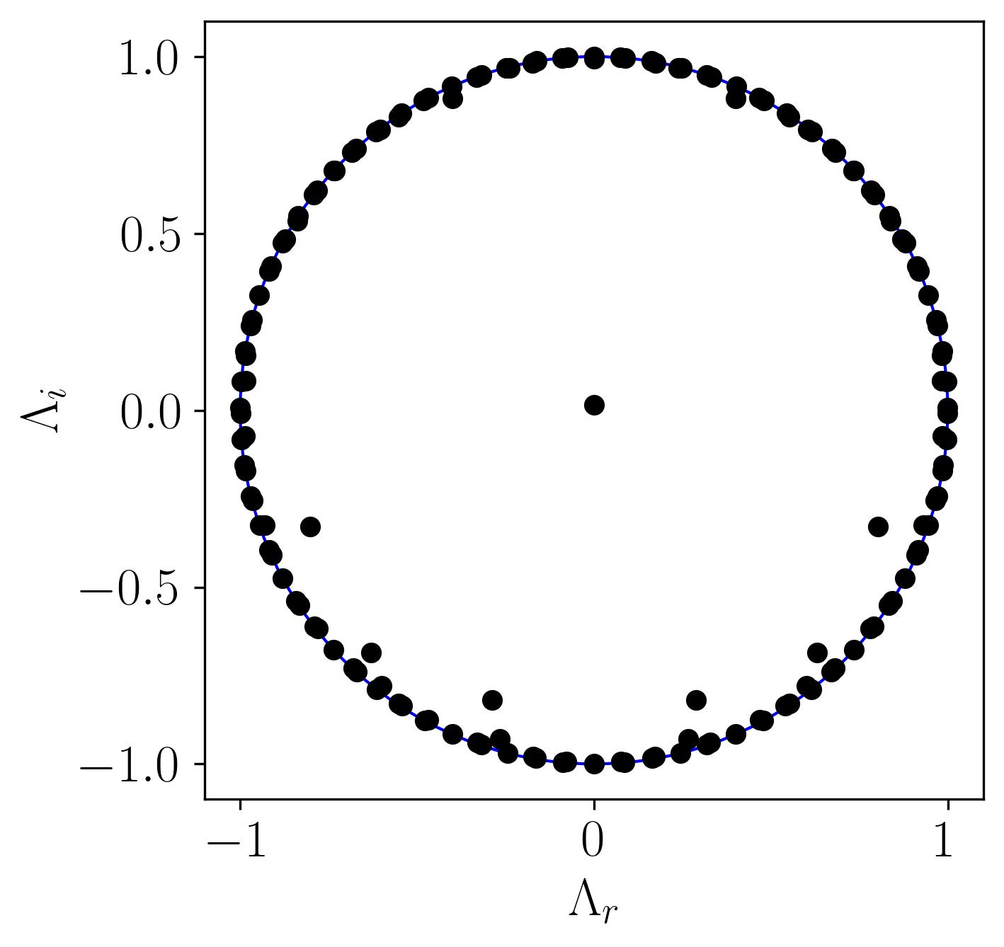
In this plot, all eigenvalues lie on the unit circle, indicating that the corresponding DMD modes are neutrally stable. These modes neither grow nor decay, making them ideal for studying steady oscillatory phenomena in the flow. This stability is particularly significant when analyzing flows where sustained oscillations dominate, such as vortex shedding in bluff-body wakes.

3D DMD Visualization

To visualize the 3D structures of DMD modes, we’ll leverage Python and ParaView. However, before diving into the visualization, it’s crucial to gain an understanding of the temporal dynamics of the flow using a simple Fast Fourier Transform (FFT). Unlike POD, DMD extracts both spatial and temporal structures, with each mode being associated with a specific frequency.

Given the complexity of a highly three-dimensional flow like ours, we aim to identify modes corresponding to distinct frequencies that signify key flow phenomena. For instance, in the case of flow around a square cylinder, periodic vortex shedding is a prominent feature in the wake. By focusing on the dominant frequency of this shedding and its harmonics, we can extract and analyze DMD modes relevant to these phenomena.

To begin, we perform an FFT to analyze the temporal dynamics of the flow:

### FFT 

### Constants
d = 0.1
Ub = 0.039
dt = 0.05*25
fs = 1/dt

Signal1 = data_Vort[50000,:]

### PSD using welch
f1, Eu1 = sp.signal.welch(Signal1, fs, nfft = len(Signal1), nperseg=len(Signal1), window='hamming')
St1 = f1*d/Ub

fig, ax = plt.subplots()

ax.loglog(St1, Eu1, label = (r'$\bf E_x$'))

xmax = St1[np.argmax(Eu1*f1/(Ub**2))]
print("Strouhal Number = ", xmax)

ax.axvline(xmax, c='r', ls='--', lw=0.8)

ax.legend(loc='best', frameon = False); # or 'best', 'upper right', etc
ax.set_xlabel(r'$St$')
ax.set_ylabel(r'$E_{u_i}$')
ax.xaxis.set_tick_params(direction='in', which='both')
ax.yaxis.set_tick_params(direction='in', which='both')
ax.xaxis.set_ticks_position('both')
ax.yaxis.set_ticks_position('both')

plt.show()

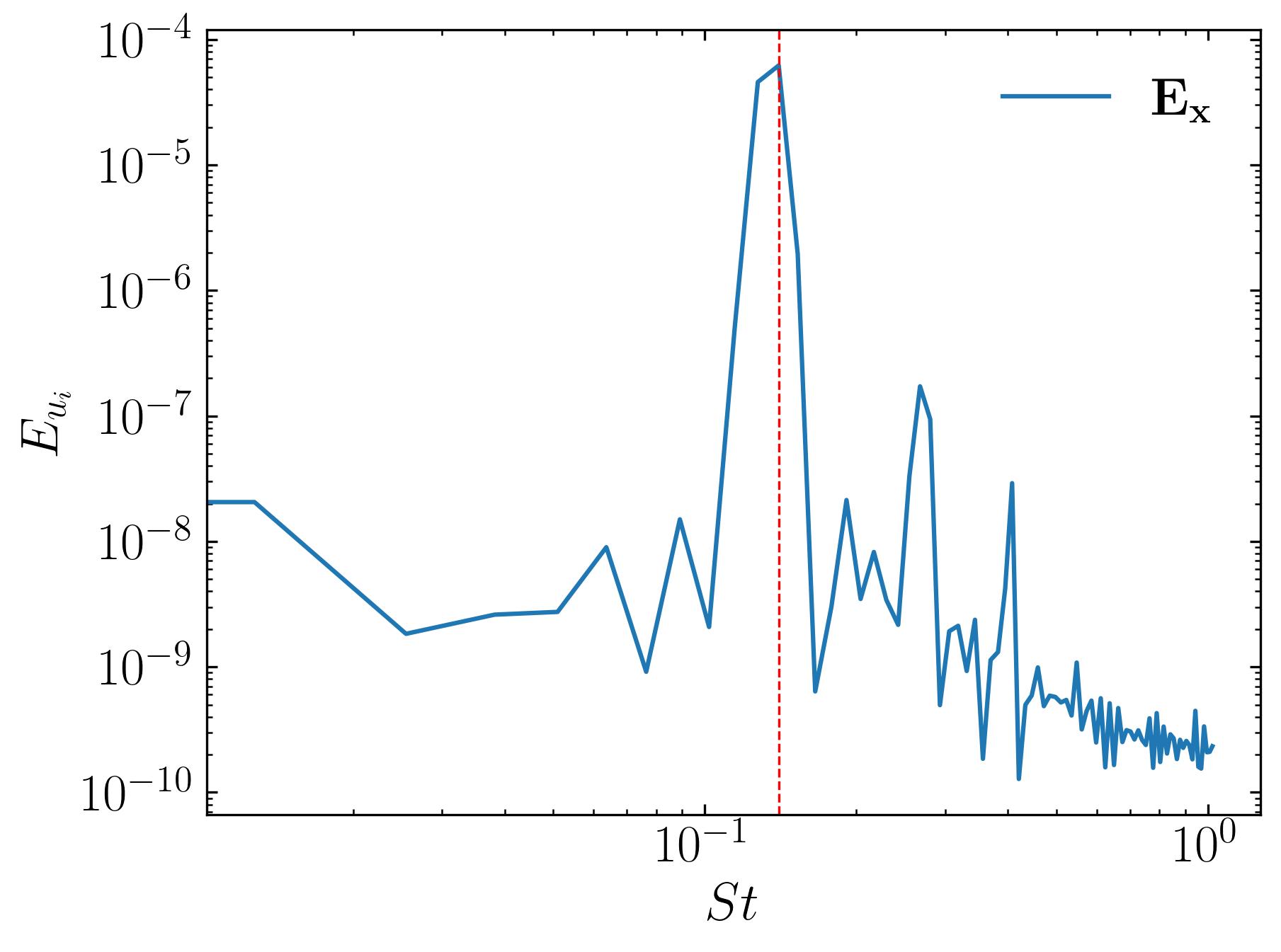
Here, we observe a dominant peak in the frequency spectrum corresponding to a Strouhal number of approximately 0.14, indicating the periodic vortex shedding in the wake. This provides a clear target for analysis: we can extract DMD modes corresponding to this frequency and its harmonics, which encapsulate the spatial structures associated with this flow phenomenon.

# File location to write a VTK File
WhereWrite = 'E:/Blog_Posts/Simulations/3D_Bai/postProcessing/'

# First snapshot, base file
WriteFile = pv.read(Surfaces + Files[0] + '/internal.vtu')

# Extract Modes
DMD_Mode1 = np.real(Phi_D[:,18]*(d/Ub))
DMD_Mode2 = np.real(Phi_D[:,19]*(d/Ub))
DMD_Mode3 = np.real(Phi_D[:,30]*(d/Ub))
DMD_Mode4 = np.real(Phi_D[:,31]*(d/Ub))
DMD_Mode5 = np.real(Phi_D[:,48]*(d/Ub))
DMD_Mode6 = np.real(Phi_D[:,49]*(d/Ub))
DMD_Mode7 = np.real(Phi_D[:,138]*(d/Ub))
DMD_Mode8 = np.real(Phi_D[:,139]*(d/Ub))

WriteFile.point_data['DMD_Mode1'] = DMD_Mode1
WriteFile.point_data['DMD_Mode2'] = DMD_Mode2
WriteFile.point_data['DMD_Mode3'] = DMD_Mode3
WriteFile.point_data['DMD_Mode4'] = DMD_Mode4
WriteFile.point_data['DMD_Mode5'] = DMD_Mode5
WriteFile.point_data['DMD_Mode6'] = DMD_Mode6
WriteFile.point_data['DMD_Mode7'] = DMD_Mode7
WriteFile.point_data['DMD_Mode8'] = DMD_Mode8

WriteFile.save(WhereWrite + 'Visualize_2.vtu')

Now, let’s open these extracted modes in ParaView to visualize their 3D structures.

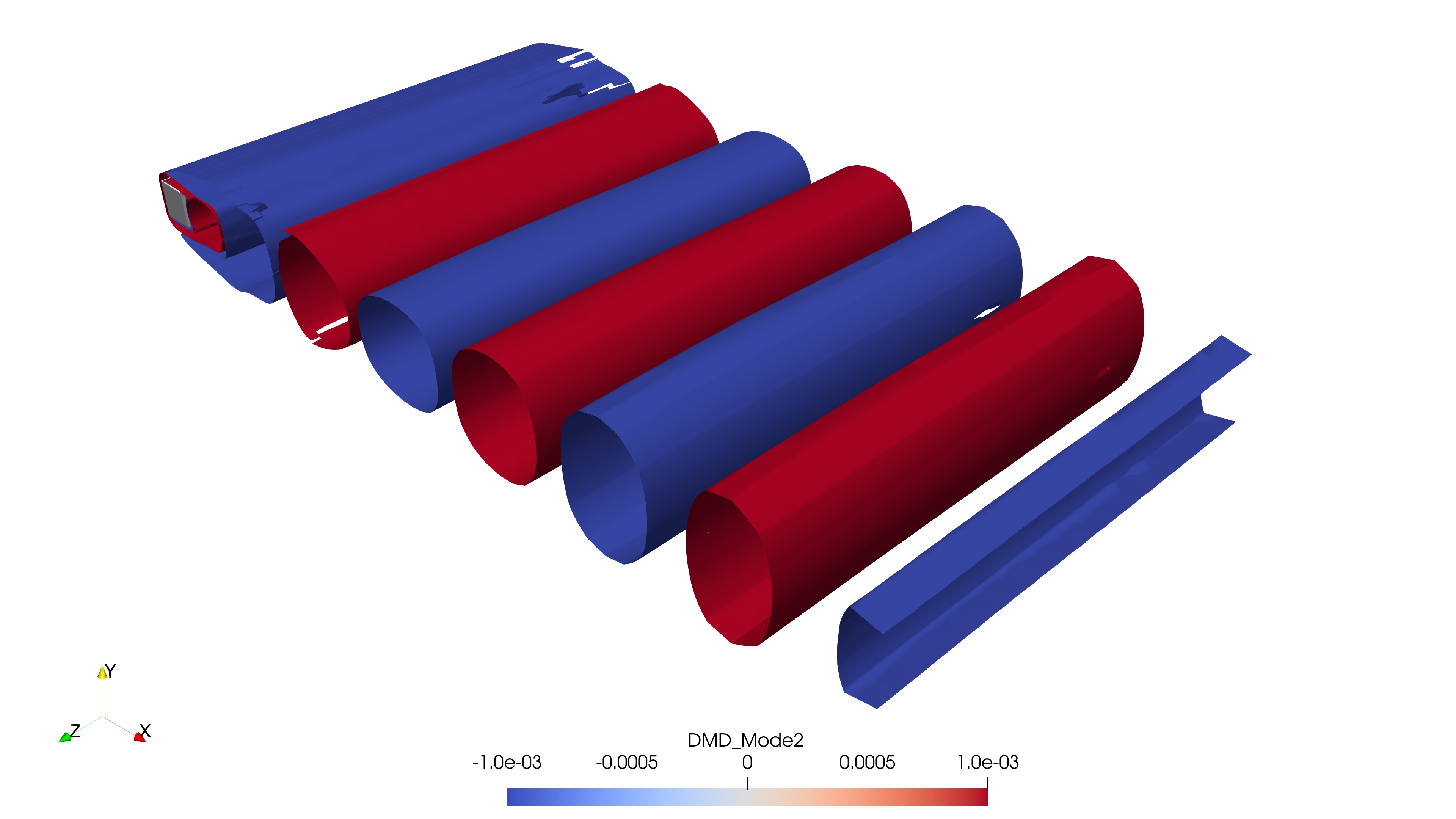
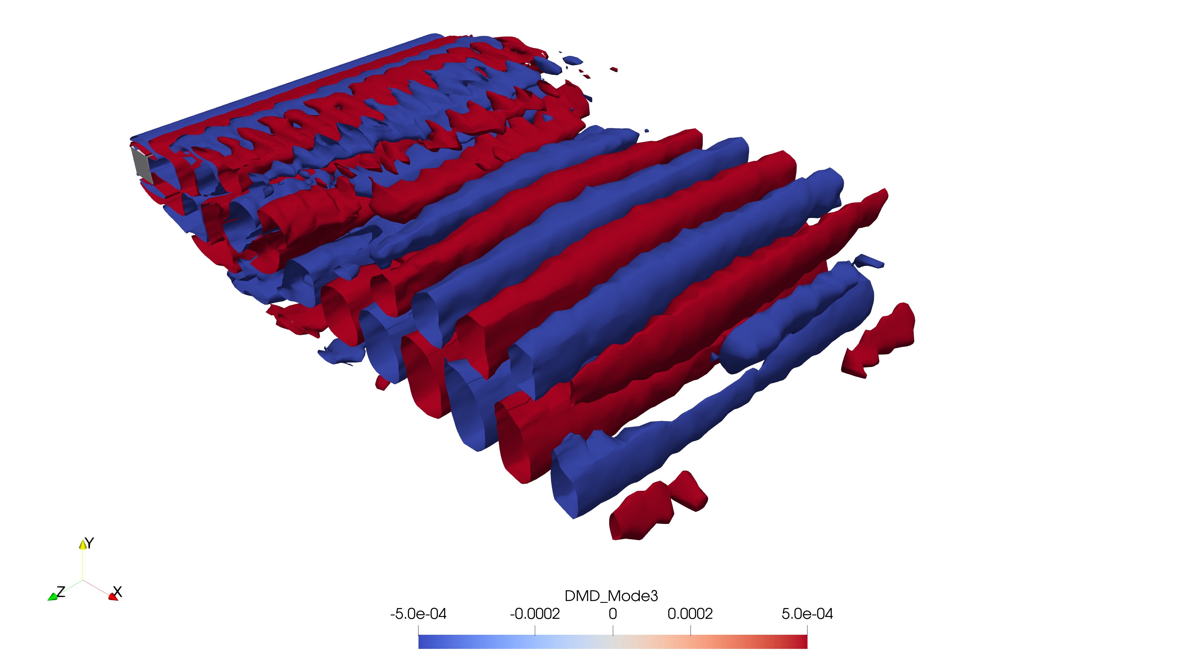
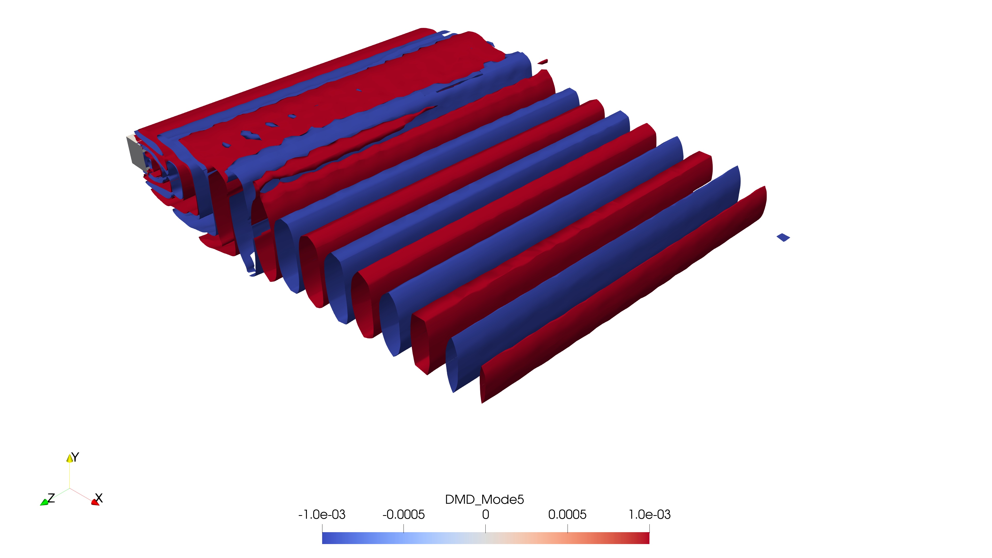
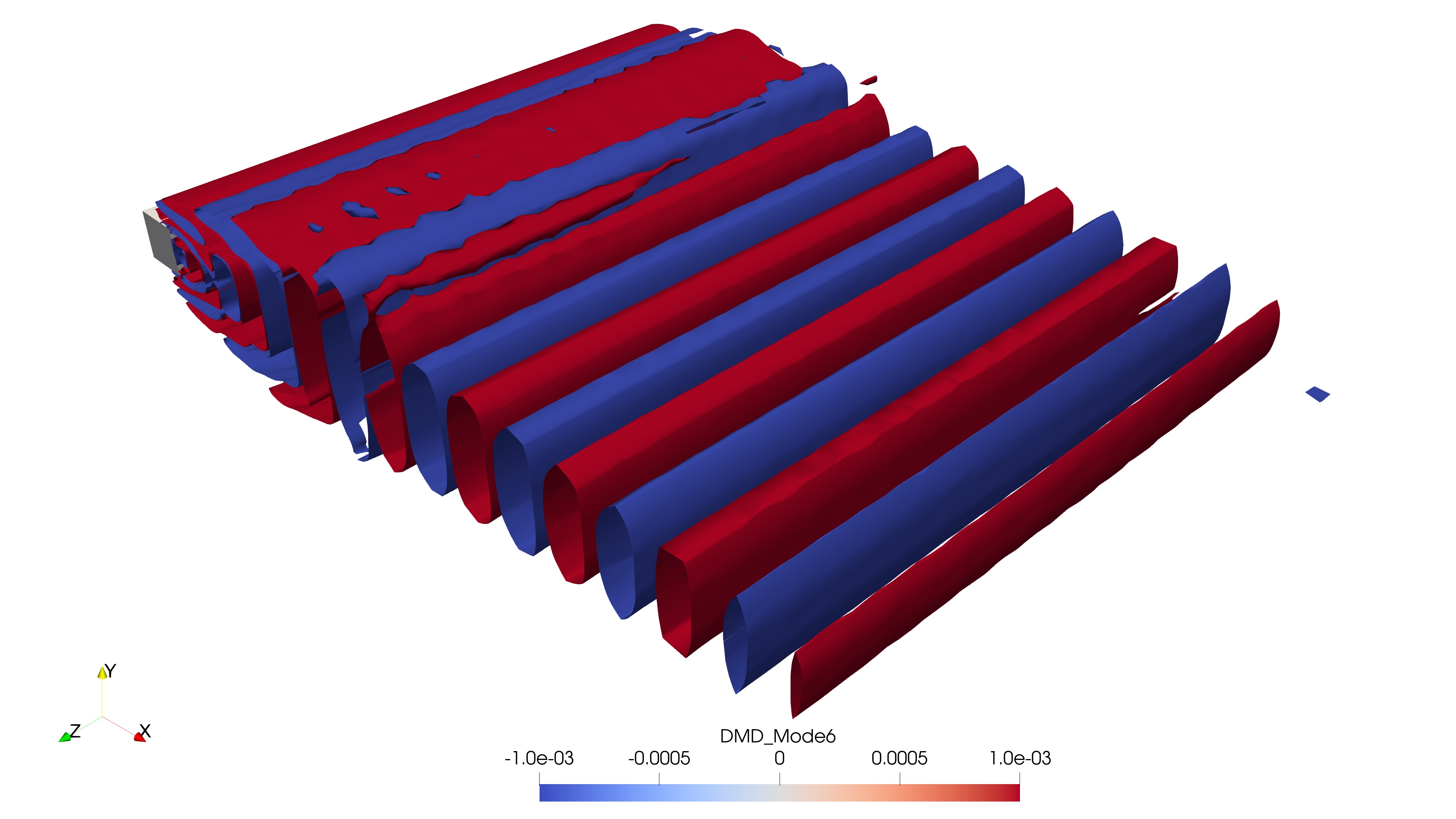
These visualizations clearly reveal the 3D flow instabilities present in the dataset. With higher-resolution data, one could delve deeper into the vortex dynamics, observe the formation of ribs and rollers, and explore complex interactions within such flows. This highlights the power of DMD in identifying and isolating key spatio-temporal features.

To gain further insights, let’s extract a 2D slice from the dataset and use Python for a more detailed visualization of the flow structures behind the cylinder. Using ParaView, create and save the slice as Slice2.vtp. Then, load this slice into the Python workflow as follows:

# Read Slice
Data2D = pv.read(WhereWrite + 'Slice2.vtp')
grid = Data2D.points
x = grid[:,0]
y = grid[:,1]
z = grid[:,2]
rows, columns = np.shape(grid)
print('rows = ', rows, 'columns = ', columns)

# Extract DMD Modes inforation
DMD_Mode0 = Data2D.point_data['DMD_Mode0']
DMD_Mode1 = Data2D.point_data['DMD_Mode1']
DMD_Mode2 = Data2D.point_data['DMD_Mode2']
DMD_Mode3 = Data2D.point_data['DMD_Mode3']
DMD_Mode4 = Data2D.point_data['DMD_Mode4']
DMD_Mode5 = Data2D.point_data['DMD_Mode5']
DMD_Mode6 = Data2D.point_data['DMD_Mode6']
DMD_Mode7 = Data2D.point_data['DMD_Mode7']
DMD_Mode8 = Data2D.point_data['DMD_Mode8']

Finally, we can plot the selected modes for a clear visualization of the 2D flow structures:

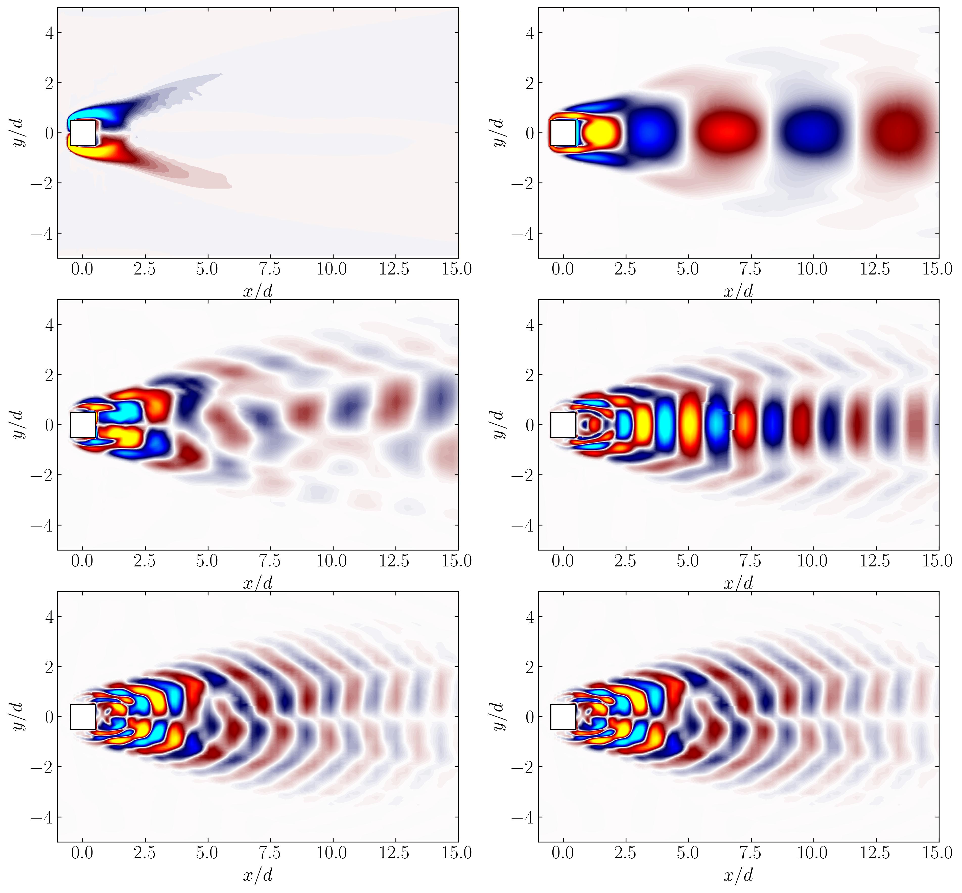
In this article, we explored the application of 3D Dynamic Mode Decomposition (DMD) to unravel the spatio-temporal dynamics of a highly three-dimensional flow. From understanding the DMD spectra and its implications for dynamic behavior to visualizing 3D flow structures in ParaView, we showcased how DMD serves as a powerful tool for uncovering complex flow phenomena. By coupling this technique with Python and OpenFOAM datasets, we demonstrated a workflow that balances computational rigor with visual clarity. The ability to isolate dominant frequencies and corresponding spatial modes opens the door to deeper insights into vortex shedding, instabilities, and flow evolution. As CFD data grows richer and more intricate, tools like DMD will continue to play a pivotal role in bridging numerical simulations with actionable insights.