Simulating real-world fluid dynamics problems often requires the ability to handle dynamic changes in the computational domain. OpenFOAM’s dynamic mesh capabilities provide the necessary tools for this purpose. This blog explores the fascinating concept of dynamic mesh motion in OpenFOAM, specifically the mesh deformation method using prescribed motion technique. I will showcase the case setup and provide a general overview of simulating mesh motion in OpenFOAM.

Simulating real-world fluid dynamics often requires accounting for moving boundaries, deformable structures, or objects in motion. These scenarios introduce significant challenges in numerical modeling, especially in maintaining the accuracy and stability of simulations. OpenFOAM addresses these challenges with its dynamic mesh capabilities. Dynamic meshes allow for the computational grid to evolve over time, adapting to changes in geometry or boundary motion. Among the various techniques available, the prescribed mesh motion method offers a robust way to model scenarios where the motion is predetermined, such as the periodic oscillation of a valve, the movement of a robotic arm, or the deformation of a piston. This approach enables precise control over mesh deformation, ensuring that the computational domain accurately represents the physical system at every timestep.

In this blog, I will explore dynamic mesh motion with a focus on the prescribed mesh motion method. This approach is particularly useful when the motion of an object or boundary is predefined. To illustrate this, we will use the example of flow around a square cylinder at a Reynolds number of 100, where the cylinder is subjected to prescribed motion. Through this practical case study, we aim to demystify dynamic mesh motion and equip you with the tools to implement it in OpenFOAM simulations. To follow along, download the case setup from here.

Lets Begin!!!

Understanding Dynamic Mesh Motion

Dynamic mesh motion refers to the ability of the computational mesh to adapt and move in response to changes in boundary positions or object movements. This capability is essential for accurately capturing the interaction between fluid flow and moving geometries.

In OpenFOAM, dynamic mesh motion can be categorized into several methods, including:

1. Prescribed Motion: The motion is explicitly defined by the user, such as a sine wave or a linear translation.
2. Solver-Based Motion: The motion is determined by solving a set of equations, typically for fluid-structure interaction (FSI) problems.
3. Mesh Topology Changes: This involves adding or removing cells during the simulation, commonly used in overset or sliding meshes.

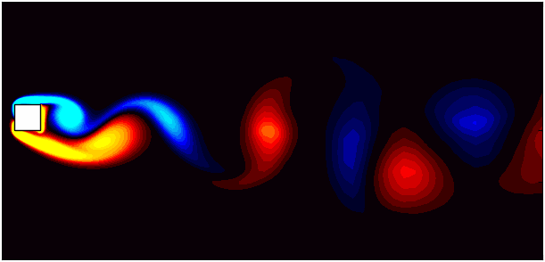
This blog focuses on the prescribed motion method, where the motion is user-defined and implemented using the dynamicMeshDict. This method is computationally efficient and straightforward to use for scenarios where the motion pattern is known a priori. For this I will use the flow around a square cylinder as the base case. The flow around a square cylinder is a classic CFD problem often used to study vortex shedding phenomena and wake dynamics. At a Reynolds number of 100, the flow is laminar, and the cylinder exhibits periodic vortex shedding in its wake. By introducing prescribed motion to the cylinder, we add complexity to the simulation, making it an excellent case for demonstrating dynamic mesh capabilities.

The cylinder’s motion is prescribed as a sinusoidal oscillation in the transverse direction, defined by the equation:

where, A is the amplitude, $\omega = 2\pi f$ is the angular frequency, and t is the time.

To accurately capture the interaction between the oscillating cylinder and the surrounding fluid, the mesh must deform dynamically while maintaining high quality. Using the prescribed motion method in OpenFOAM, we can define the cylinder’s oscillation and simulate the flow field with precision.

Dynamic Mesh Configuration in OpenFOAM

To enable dynamic mesh motion in OpenFOAM, specific settings must be configured to govern how the mesh adapts to the prescribed motion of the cylinder. This process involves modifying several files in the case directory to define the motion and ensure consistency across the setup. In total, the following four changes are required:

1. Add a dynamicMeshDict file in the Case/constant/ directory to define the dynamic mesh solver and motion type.
2. Specify motion definitions in boundary conditions, using either the pointDisplacement or motionUx file, depending on the motion type.
3. Adjust boundary conditions in the velocity field to account for the movement of the cylinder.
4. Include cellDisplacement settings in the Case/system/fvSolution file to solve the mesh motion equation.

Let’s go through each of these changes step-by-step.

Defining the Motion Solver

To configure the motion solver, the Case/constant/dynamicMeshDict file is modified to specify the dynamic mesh settings. Below is an example configuration:

// * * * * * * * * * * * * * * * * * * * * * * * * * * * * * * * * * * * * * //

dynamicFvMesh      dynamicMotionSolverFvMesh;

motionSolverLibs ("libfvMotionSolvers.so");

motionSolver            displacementLaplacian;

displacementLaplacianCoeffs 
{
    diffusivity         inverseDistance	(PRISM);
}

// ************************************************************************* //

Here, dynamicFvMesh specifies the type of dynamic mesh to use. dynamicMotionSolverFvMesh indicates that a motion solver will be used to compute the mesh deformation. For the motionSolver, displacementLaplacian solver is selected, which calculates mesh motion by solving a Laplace equation for point displacements or velocities. Under the displacementLaplacianCoeffs, diffusivity determines how mesh motion is distributed. The inverseDistance option ensures smoother deformation near the moving boundary. The diffusivity model (inverseDistance) ensures that mesh deformation diminishes with increasing distance from the moving boundary, minimizing distortion in the outer regions of the mesh. If the displacement-based method is chosen (displacementLaplacian), a pointDisplacement boundary condition must be set up to prescribe motion on relevant boundaries.

Specifying the Motion

The motion of the mesh is defined in the pointDisplacement file within the Case/0/ directory. This file specifies the boundary conditions for the prescribed motion. Below is the configuration for the oscillating motion of the cylinder:

  PRISM
  {
      type            oscillatingDisplacement;
      amplitude       ( 0 0.05 0 );
      omega           6.28318;
      value           uniform ( 0 0 0 );
  }

As noted earlier, the motion we are prescribing is a sinusoidal wave defined by an amplitude and angular frequency. I will chose the amplitude to be 0.05 in Y direction, and a frequency of 1, making the angular frequency (omega) to be $2\pi$.

The remaining parts of the domain, which are stationary, should be assigned a fixedValue boundary condition. This ensures no motion occurs in these regions.

Below is an example configuration for the non-moving boundaries:

/*--------------------------------*- C++ -*----------------------------------*\
| =========                 |                                                 |
| \\      /  F ield         | OpenFOAM: The Open Source CFD Toolbox           |
|  \\    /   O peration     | Version:  v2312                                 |
|   \\  /    A nd           | Website:  www.openfoam.com                      |
|    \\/     M anipulation  |                                                 |
\*---------------------------------------------------------------------------*/
FoamFile
{
    version     2.0;
    format      ascii;
    class       pointVectorField;
    object      pointDisplacement;
}
// * * * * * * * * * * * * * * * * * * * * * * * * * * * * * * * * * * * * * //

dimensions      [0 1 0 0 0 0 0];

internalField   uniform (0 0 0);

boundaryField
{
	TOP
    {
        type            fixedValue;
        value           uniform (0 0 0);
    }
    BOTTOM
    {
        type            fixedValue;
        value           uniform (0 0 0);
    }

    SIDE1
    {
        type            empty;
    }
    SIDE2
    {
        type            empty;
    }

    INLET
    {
        type            fixedValue;
        value           uniform (0 0 0);
    }

    OUTLET
    {      
        type            fixedValue;
        value           uniform (0 0 0);
    }

    PRISM
    {
        type            oscillatingDisplacement;
        amplitude       ( 0 0.05 0 );
        omega           6.28318;
        value           uniform ( 0 0 0 );
    }
	
}

// ************************************************************************* //

Modify other boundary conditions

Next, we need to adjust the velocity boundary conditions for the moving cylinder. To account for the motion of the cylinder, the boundary condition for the cylinder’s surface should be set to movingWallVelocity as shown below:

  PRISM
  {
    type                      movingWallVelocity;
    value                     uniform (0 0 0);
  }

For other boundaries such as the inlet and outlet, the velocity boundary conditions need to account for the moving mesh. Depending on the scenario, you may use velocity boundary conditions like inletVelocity or outletVelocity, as appropriate for the specific problem. To avoid creating unrealistic pressure gradients at the cylinder surface, the pressure boundary condition should be set to zeroGradient on the cylinder:

   PRISM
  {
      type            zeroGradient;
  }

Add mesh motion linear solver

Dynamic meshes can degrade in quality as the simulation progresses, leading to issues such as excessive skewness or non-orthogonality in the mesh. To mitigate these issues, it is essential to configure the linear solver settings and mesh-quality constraints in the fvSolution file. Below is an example of the required settings to ensure stable mesh motion and maintain mesh quality:

    cellDisplacement
    {
        solver          PCG;
        preconditioner  DIC;
        tolerance       1e-08;
        relTol          0;
		    minIter		3;
    }
	
	  cellDisplacementFinal
    {
        $cellDisplacement;
        relTol          0;
    }

Running the Simulation

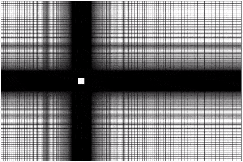
After completing the configuration, it’s important to check the quality of the mesh before starting the simulation. You can use the checkMesh utility to assess the mesh quality and ensure that there are no issues such as skewness, non-orthogonality, or overly deformed cells. Once the mesh passes the check, you can preview the motion of the mesh using the moveDynamicMesh utility. This allows you to confirm that the mesh deforms correctly before solving the flow equations.

To preview the motion without solving for the flow, you can set a small time-step in the controlDict file, ensuring the time-step adheres to the CFL criterion (for example, a value of 0.4 ensures proper temporal refinement). If needed, you can also run the moveDynamicMesh utility with a larger time-step to get a quicker preview. Open up your case into an OpenFOAM sourced terminal and type in:

moveDynamicMesh

The output should look something like this:

Create time

Create dynamic mesh for time = 0
Selecting dynamicFvMesh dynamicMotionSolverFvMesh
Selecting motion solver: displacementLaplacian
Applying motion to entire mesh
Selecting motion diffusion: inverseDistance
Selecting patchDistMethod meshWave


PIMPLE: Operating solver in PISO mode

Time = 0.0004
PIMPLE: iteration 1
DICPCG:  Solving for cellDisplacementx:  solution singularity
DICPCG:  Solving for cellDisplacementy, Initial residual = 1, Final residual = 4.9321443e-14, No Iterations 3
    Point usage OK.
    Upper triangular ordering OK.
    Topological cell zip-up check OK.
    Face vertices OK.
    Face-face connectivity OK.
    Mesh topology OK.
    Boundary openness (-6.8575785e-18 1.3863136e-17 1.0085072e-15) OK.
    Max cell openness = 2.5540133e-16 OK.
    Max aspect ratio = 100.84633 OK.
    Minimum face area = 9.9295354e-07. Maximum face area = 0.006908216.  Face area magnitudes OK.
    Min volume = 9.9295355e-08. Max volume = 0.00023747556.  Total volume = 0.86300005.  Cell volumes OK.
    Mesh non-orthogonality Max: 1.3579948 average: 0.0780059
    Non-orthogonality check OK.
    Face pyramids OK.
    Max skewness = 0.0064898452 OK.
    Mesh geometry OK.
Mesh OK.
ExecutionTime = 1.56 s  ClockTime = 2 s

...

You can write out the time directories at regular intervals to visualize the animation of the mesh motion. This helps in confirming the smoothness and accuracy of the mesh deformation as the simulation progresses. To do so, include the following in your controlDict:

writeInterval    50;  // Write the data every 50 time steps

You can then visualize the results using software like ParaView to create an animation of the mesh motion.

Once you are satisfied with the mesh motion and the preview looks good, you can proceed to run the solver. Use the pimpleFoam command to simulate the flow around the moving cylinder. This will solve the flow field while accounting for the dynamic motion of the mesh.

Challenges and Best Practices

Challenges:

1. Mesh Quality Maintenance: Dynamic meshes can lead to highly skewed or non-orthogonal cells, affecting solution accuracy and stability. Excessive deformation may result in solver divergence.
2. Computational Cost: Deforming meshes increase computational overhead, particularly for complex motions or high-resolution grids.
3. Boundary Condition Complexity: Defining accurate boundary conditions for moving boundaries can be challenging, especially for coupled systems.

Best Practices:

1. Pre-Simulation Checks: Use checkMesh and moveDynamicMesh to verify the mesh quality and motion before running the simulation. Start with a coarse mesh to debug motion and refine later for accuracy.
2. Mesh Quality Controls: Set strict mesh quality criteria in the fvSolution file to avoid excessive skewness or stretching. Regularly monitor mesh quality during the simulation.
3. Solver Selection and Settings: Choose solvers like pimpleFoam with relaxation factors to improve stability for dynamic simulations. Use adaptive timesteps to maintain an appropriate Courant number.