Python Tools for Analyzing and Visualizing Mesh Motion Simulations
Postprocessing is a critical step in any simulation workflow, providing insights into the results and enabling effective communication of findings. When it comes to dynamic mesh motion simulations, visualizing the mesh deformation and understanding its effects on flow features can be particularly challenging. In this article, I’ll explore how to use Python for postprocessing such simulations, focusing on extracting, analyzing, and visualizing mesh motion data. With a combination of powerful libraries like Matplotlib, NumPy, and PyVista, we’ll unlock techniques to create meaningful visualizations and derive valuable insights from simulation results.
Dynamic mesh motion simulations provide valuable insights into the interaction between moving boundaries and the surrounding flow. However, the true potential of these simulations is realized only through effective postprocessing, where mesh behavior is analyzed and visualized. In this blog, we’ll focus on extracting, visualizing, and analyzing mesh motion data using Python, showcasing practical techniques to interpret complex deformations and movements. Building on the foundational tutorials from my previous blogs on setting up mesh motion simulations, this article will guide you through postprocessing workflows, enabling you to transform raw data into actionable insights.
II will build upon the tutorial cases introduced in my previous two articles. These include the simulation of flow around a heaving square cylinder (Available here) and flow around a thin flat plate aligned parallel to the flow direction (download here).
Lets Begin!!!
Setting Up the Environment
Before diving into postprocessing, ensure your environment is ready to handle the data efficiently. This involves installing essential Python libraries like:
-
numpyfor numerical operations, -
matplotlibfor creating static and animated visualizations, -
pyvistafor handling and visualizing mesh data in 3D, and -
vtkfor working with VTK-formatted files.
For setting up your Python environment, refer to my previous article.
Here’s how you can set up the environment:
pip install numpy matplotlib pyvista vtk
Understanding motion kinematics
Beyond visualization, quantitative analysis can provide deeper insights into the dynamics of mesh motion. For instance, by visualizing the kinematics of mesh motion using Python, you can estimate the period of one pitching or heaving cycle and determine appropriate intervals for data writing. To get started, open a Jupyter notebook and import the necessary modules:
import matplotlib.colors
import matplotlib.pyplot as plt
import numpy as np
import pandas as pd
import fluidfoam as fl
import scipy as sp
import os
import matplotlib.animation as animation
import pyvista as pv
import imageio
import io
%matplotlib inline

plt.rcParams.update({'font.size' : 18, 'font.family' : 'Times New Roman', "text.usetex": True})
cmap = matplotlib.colors.LinearSegmentedColormap.from_list("", ["cyan", "xkcd:azure", "blue", "xkcd:dark blue", "white", "xkcd:dark red", "red", "orange", "yellow"])
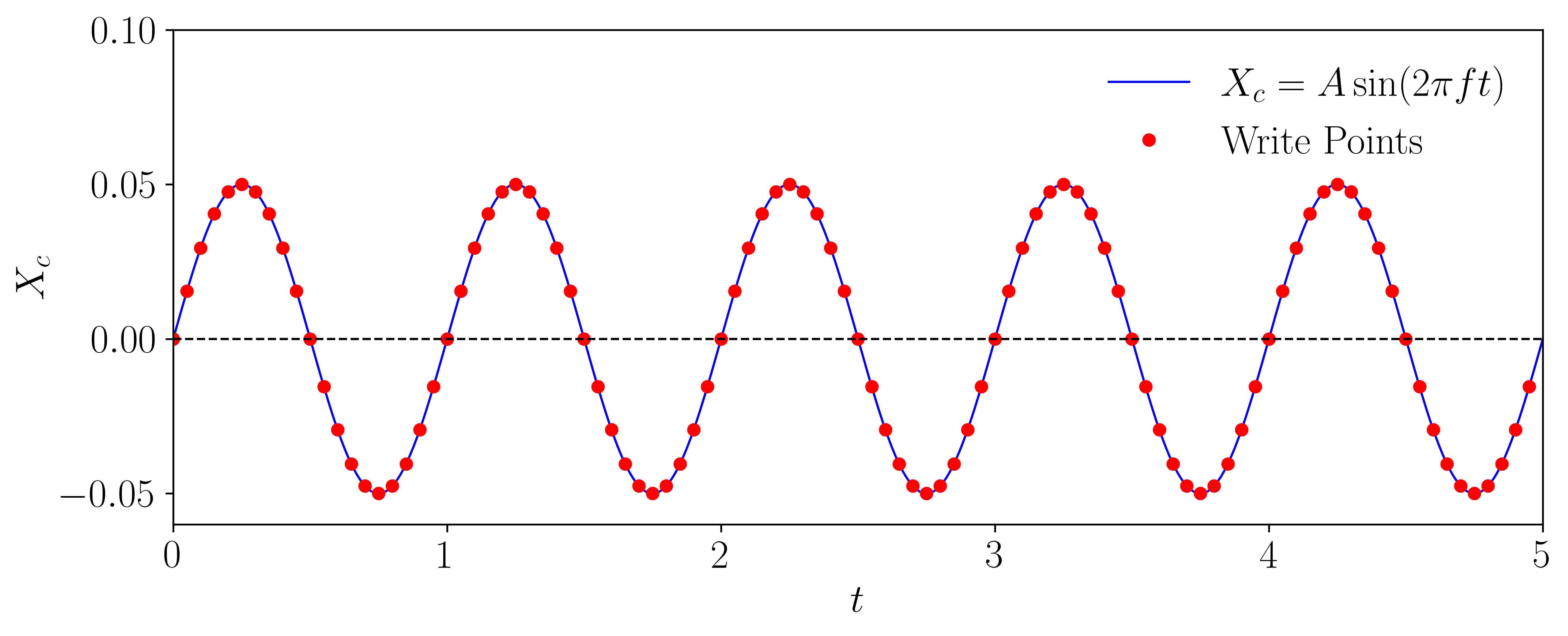
The motion we aim to prescribe follows a sinusoidal wave, mathematically represented as:
\[y(t) = A sin(\omega t)\]To define the motion, let’s specify the amplitude (A) and the frequency (f) of the sinusoidal wave:
# Motion Xc = A Sin(2*pi*f*t)
A = 0.05
f = 1
omega = 2*np.pi*f
Times = np.arange(0, 5, 0.0004)
Xc = A*np.sin(omega*Times)
Finally, we can plot the motion equation along with markers representing the time intervals at which data will be saved in OpenFOAM:
# Plot
fig, ax = plt.subplots(figsize = (11, 4))
ax.plot(Times, Xc, label = r'$X_c = A \sin(2\pi f t)$', color = 'blue', linewidth = 1)
MarkEvery = 125
ax.plot(Times, Xc, 'ro', markersize = 5, label = 'Write Points', markevery = MarkEvery)
ax.axhline(y = 0, color = 'black', linestyle = '--', linewidth = 1)
ax.legend(loc='best', frameon = False); # or 'best', 'upper right', etc
ax.set_xlim([0, 5])
ax.set_ylim([-0.06, 0.1])
ax.set_ylabel(r'$X_c$')
ax.set_xlabel(r'$t$')
plt.show()
By visualizing this plot, you can observe the sinusoidal motion profile and identify the specific time intervals for data saving. This approach ensures that the data is captured consistently and aligns with the prescribed motion.
Extracting Mesh Data
The first step in postprocessing is to extract mesh motion data from your simulation. OpenFOAM typically provides this information as displacement fields (pointDisplacement) or velocity fields (motionUx), which can be processed further. For 2D simulations, the foamToVTK utility simplifies this process by converting OpenFOAM case data into VTK format, making it easier to handle in Python. Once converted, you can use Python libraries like pyvista to load and manipulate the data.
However, not all simulations are strictly 2D, and extracting meaningful slices or surfaces from 3D simulations is often necessary. OpenFOAM offers an efficient way to achieve this using the surfaces function object. This tool allows you to extract two-dimensional slices or surfaces from the dataset. To configure it, create a file named <Case>/system/surfaces and set it up as shown below:
surfaces
{
    type            surfaces;
    libs            ("libsampling.so");
    writeControl   	timeStep;
    writeInterval   10;

    surfaceFormat   vtk;
    fields          (p U);

    interpolationScheme cellPoint;

    surfaces
    {
        zNormal
        {
            type        cuttingPlane;
            point       (0 0 0.05);
            normal      (0 0 1);
            interpolate true;
        }
    };
};
You can use this function object during runtime to extract surfaces at specified writeIntervals, or, as in this case, use it as a postprocessing tool after completing your simulation. For instance, if your simulation has reached statistical convergence, you can save surfaces for 50 time directories as follows:
goswami@ME:/mnt/f/Moving_Meshes_OFTest/Org/Org$ ls
0        4.56315  4.96315  5.36315  5.76315  6.16315  6.56315  6.96315  7.36315  7.76315  8.16315
4.24315  4.64315  5.04315  5.44315  5.84315  6.24315  6.64315  7.04315  7.44315  7.84315  constant
4.32315  4.72315  5.12315  5.52315  5.92315  6.32315  6.72315  7.12315  7.52315  7.92315  foam.foam
4.40315  4.80315  5.20315  5.60315  6.00315  6.40315  6.80315  7.20315  7.60315  8.00315  system
4.48315  4.88315  5.28315  5.68315  6.08315  6.48315  6.88315  7.28315  7.68315  8.08315
Once your case is set up, open an OpenFOAM-sourced terminal and execute the following command:
pimpleFoam -postProcess -func surfaces
This command will process the simulation results and write the pressure and velocity data for the specified slice at each time directory. The output will be stored in the <Case>/postProcessing/surfaces/ directory. A sample output might look like this:
goswami@ME:/mnt/f/Moving_Meshes_OFTest/Org/Org/postProcessing/surfaces$ ls
4.24315  4.56315  4.88315  5.20315  5.52315  5.84315  6.16315  6.48315  6.80315  7.12315  7.44315  7.76315  8.08315
4.32315  4.64315  4.96315  5.28315  5.60315  5.92315  6.24315  6.56315  6.88315  7.20315  7.52315  7.84315  8.16315
4.40315  4.72315  5.04315  5.36315  5.68315  6.00315  6.32315  6.64315  6.96315  7.28315  7.60315  7.92315
4.48315  4.80315  5.12315  5.44315  5.76315  6.08315  6.40315  6.72315  7.04315  7.36315  7.68315  8.00315
Each time directory will contain files for the extracted surfaces. For example:
goswami@ME:/mnt/f/Moving_Meshes_OFTest/Org/Org/postProcessing/surfaces$ tree 4.24315/
4.24315/
└── zNormal.vtp
Here, zNormal.vtp is the VTK file containing the pressure and velocity data for the slice at the specified time step.
Now, let’s move to postprocessing in Python. Start by setting up the path variables and constants in your Jupyter notebook. These will help you organize and access the data efficiently in your analysis workflow.
# Path Variables
Path = 'F:/Moving_Meshes_OFTest/Org/Org/postProcessing/surfaces/'
save_path = 'F:/Moving_Meshes_OFTest/Org/'
save_Blog = 'F:/E_Drive/Blog_Posts/2025_Blogs/Blog9/'
Files = os.listdir(Path)

# Constants
d = 0.1
Ub = 1
To begin, load the data from a single VTK file using the following code:
Data = pv.read(Path + Files[0] + '/zNormal.vtp')
grid = Data.points
x = grid[:,0]
y = grid[:,1]
z = grid[:,2]
rows, columns = np.shape(grid)
print('rows = ', rows, 'columns = ', columns)
To extract and compute the vorticity for all time steps, use PyVista within a loop. This approach enables the creation of a matrix containing the vorticity data:
Data = pv.read(Path + Files[0] + '/zNormal.vtp')
grid = Data.points
x = grid[:,0]
y = grid[:,1]
z = grid[:,2]
rows, columns = np.shape(grid)
print('rows = ', rows, 'columns = ', columns)

### For U
Snaps = len(Files)
data_Vort = np.zeros((rows,Snaps-1))
grid_x = np.zeros((rows,Snaps-1))
grid_y = np.zeros((rows,Snaps-1))
grid_z = np.zeros((rows,Snaps-1))
for i in np.arange(0,Snaps-1):
    data = pv.read(Path + Files[i] + '/zNormal.vtp')
    grid = data.points
    grid_x[:,i:i+1] = np.reshape(grid[:,0], (rows,1), order='F')
    grid_y[:,i:i+1] = np.reshape(grid[:,1], (rows,1), order='F')
    grid_z[:,i:i+1] = np.reshape(grid[:,2], (rows,1), order='F')
    gradData = data.compute_derivative('U', vorticity=True)
    grad_pyvis = gradData.point_data['vorticity']
    data_Vort[:,i:i+1] = np.reshape(grad_pyvis[:,2], (rows,1), order='F')

np.save(save_path + 'VortZ.npy', data_Vort)
np.save(save_path + 'grid_x.npy', grid_x)
np.save(save_path + 'grid_y.npy', grid_y)
np.save(save_path + 'grid_z.npy', grid_z)
After extracting the data, visualize the vorticity field with a contour plot:
Contour = 0
A = 0.05/0.1
Omega = 2*np.pi

fig, ax = plt.subplots(figsize=(11, 4))
p = ax.tricontourf(grid_x[:,Contour]/0.1, grid_y[:, Contour]/0.1, data_Vort[:,Contour]*(d/Ub),
                   levels = 1001, vmin=-1.8, vmax=1.8, cmap = cmap)
patches = []
patches.append(plt.Rectangle((-0.5, (A*np.sin(Omega*float(Files[Contour])))-0.5), 1, 1,
                             ec='k', color='white', zorder=2))
ax.add_patch(patches[0])
ax.xaxis.set_tick_params(direction='in', which='both')
ax.yaxis.set_tick_params(direction='in', which='both')
ax.xaxis.set_ticks_position('both')
ax.yaxis.set_ticks_position('both')
ax.set_xlim(-1, 20)
ax.set_ylim(-5, 5)
ax.set_aspect('equal')
ax.set_xlabel(r'$x/d$')
ax.set_ylabel(r'$y/d$')
fig.set_tight_layout(True)
plt.savefig(save_Blog + 'SqCylPlot.jpeg', dpi = 600, bbox_inches = 'tight')
plt.show()
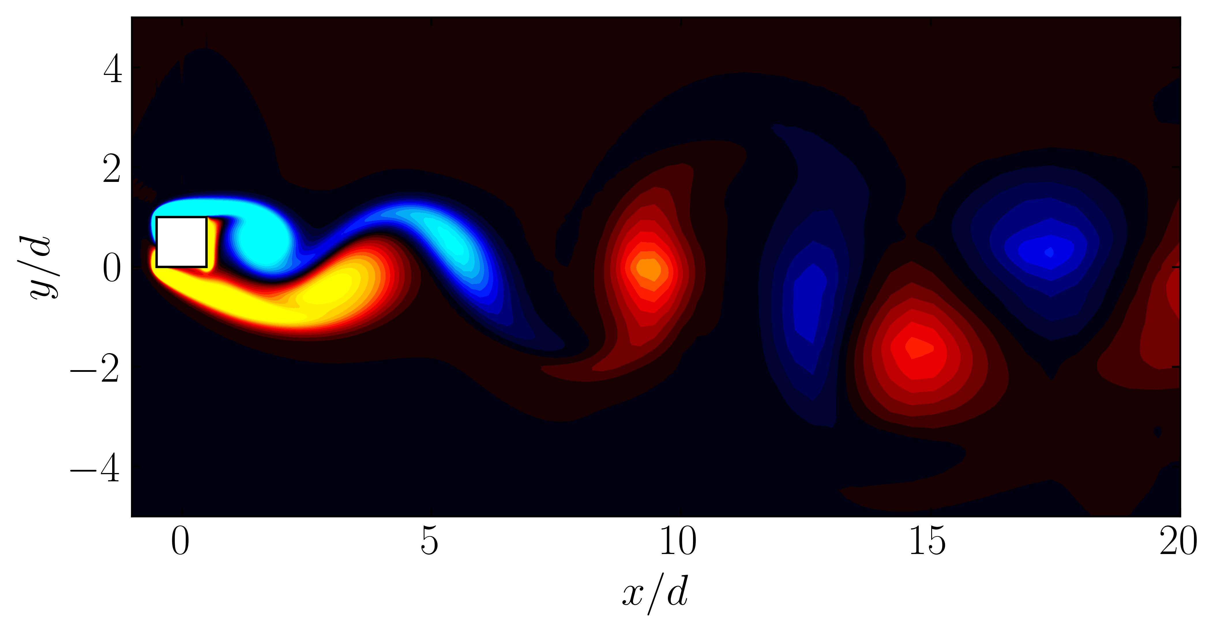
Since we are working with moving meshes, it’s crucial to account for the prescribed motion. For a sinusoidal motion, the position of the square cylinder at any time instant can be calculated using:
\[X_c = A sin(\omega T)\]This enables precise positioning of the square cylinder patch in the plot. The same process can be followed for pure pitching and pure heaving simulations.
Enjoy Reading This Article?
Here are some more articles you might like to read next: