An Introduction to Overset Mesh in OpenFOAM
Published:
Dynamic mesh motion is a critical feature in computational fluid dynamics (CFD) for simulating problems with moving boundaries or complex geometries. Among the various techniques available in OpenFOAM, the Overset mesh approach has gained popularity due to its flexibility in handling relative motion between different mesh regions. This method allows engineers and researchers to solve problems like rotor-stator interactions, aerodynamic analysis of moving vehicles, and more with enhanced accuracy and efficiency. In this blog, I’ll explore the fundamentals of Overset meshes in OpenFOAM.
In the ever-evolving field of computational fluid dynamics (CFD), the ability to simulate moving boundaries and complex geometries accurately is a game-changer. Dynamic mesh motion plays a pivotal role in enabling such simulations, with applications ranging from simulating rotating machinery to analyzing the aerodynamics of moving vehicles. OpenFOAM offers multiple approaches for dynamic mesh motion, including mesh deformation, sliding interfaces, and Overset meshes. Among these, the Overset mesh approach stands out for its ability to handle large relative motions between mesh regions while maintaining computational efficiency and accuracy. This blog explores the Overset mesh method, offering insights into its working principles.
Lets begin!!!
What is Overset Mesh?
The Overset mesh approach, also known as Chimera mesh, is a numerical technique used in CFD to simulate problems involving complex, relative motion between different parts of a domain. Unlike traditional methods such as mesh deformation, where the grid is morphed to follow the motion, or sliding interfaces, which rely on aligned interfaces, Overset mesh employs overlapping grids to model the moving and stationary parts of the domain independently.
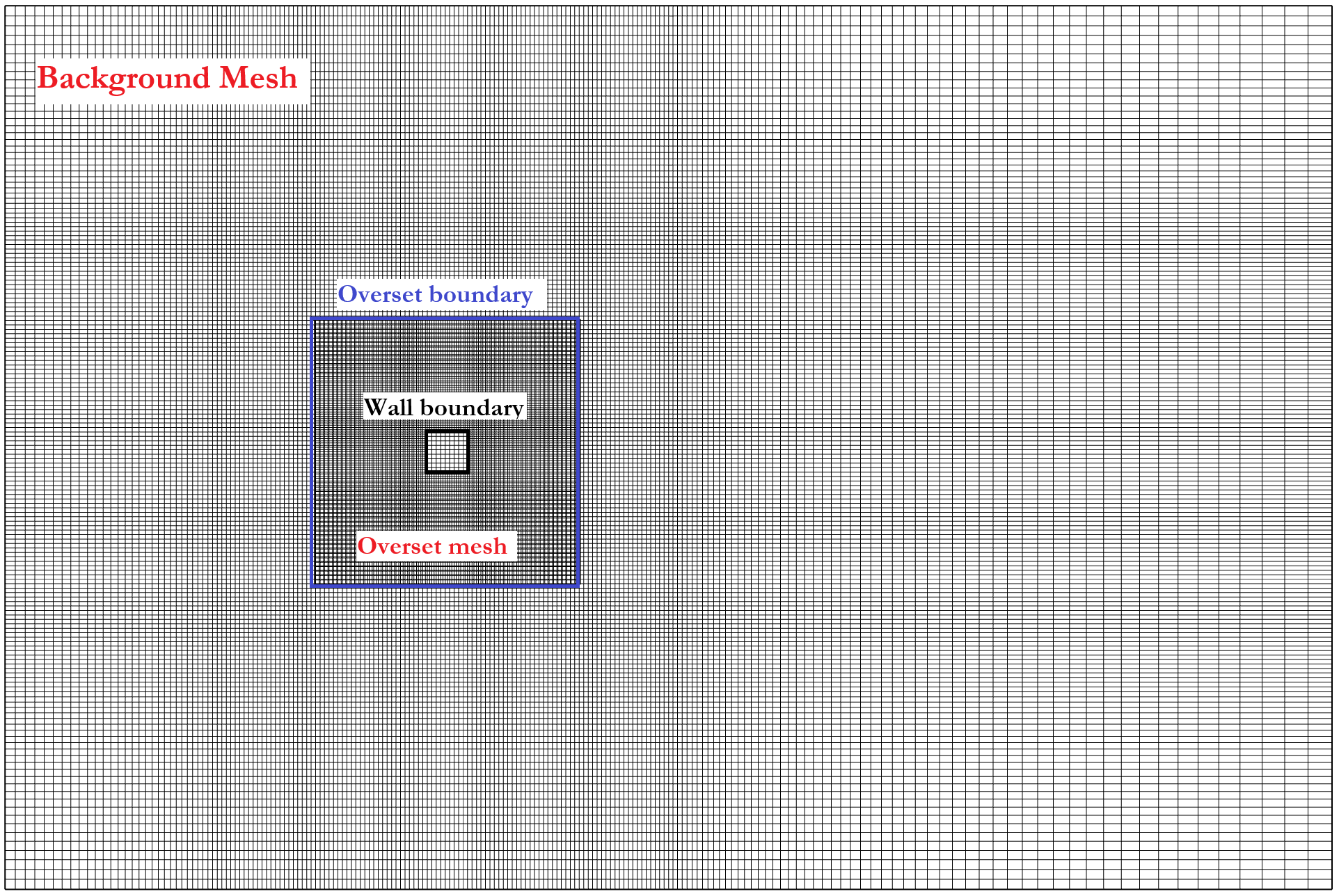
The Overset mesh approach operates on the principle of overlapping grids, which are independently defined and managed. These grids typically include a stationary background grid covering the entire computational domain and one or more foreground grids that move with the objects of interest. Unlike traditional methods, these grids do not need to conform to each other, allowing greater flexibility in simulating relative motions between different parts of the domain. The interaction between these grids is facilitated by interpolation. In the overlapping regions, field variables such as velocity and pressure are exchanged between grids through an interpolation process that ensures continuity and consistency of the solution across the domain.
A key feature of the Overset mesh approach is hole cutting, where portions of the background mesh that lie within the physical boundaries of a moving object are deactivated or marked as hole cells. This ensures that the computational effort is focused only on the relevant parts of the domain. By keeping each mesh independent, the Overset method avoids common challenges such as grid deformation and interface alignment. This independence makes it particularly suitable for problems involving large displacements, rotations, or highly complex geometries, where traditional methods may struggle.
Advantages of Overset Mesh
- Flexibility in Motion: Allows for arbitrary motions, including translations, rotations, or combinations thereof, without compromising mesh quality.
- Ease of Grid Generation: Independent grids simplify the meshing process, especially for geometries with intricate shapes or components.
- Reusability: Grids for moving parts can be reused across multiple simulations, saving time in preprocessing.
Limitations
- Computational Overhead: The interpolation process introduces additional computational cost.
- Accuracy Concerns: Interpolation errors may arise, particularly in regions with steep gradients or inadequate grid resolution.
- Complex Setup: Requires careful planning for grid placement, overlap, and boundary conditions to avoid solver instability.
Comparison with Other Techniques
The Overset mesh approach is particularly advantageous when other methods struggle, such as when simulating aircraft in flight, propeller blades, or moving objects in fluid flow.
| Feature | Mesh Deformation | Sliding Interfaces | Overset Mesh |
|---|---|---|---|
| Motion Flexibility | Limited to small deformations | Restricted to specific planes | Arbitrary large motions |
| Mesh Quality | Degrades with deformation | Maintains quality | Independent of motion |
| Setup Complexity | Moderate | Low | High |
| Computational Cost | Low | Moderate | High |
| Ideal Applications | Small displacements or deformations | Rotating machinery with fixed planes | Arbitrary motion of complex objects |
How does Overset mesh work ?
In overlapping regions, the grids communicate by exchanging information through interpolation. The cells providing this information are known as donor cells, while those receiving it are called receptor cells. This interpolation process ensures that the solution remains continuous and consistent across the grid interfaces, enabling accurate modeling of interactions between stationary and moving regions.
An essential step in Overset mesh simulations is hole cutting. In this process, the solver identifies and deactivates portions of the background grid that fall within the physical boundaries of a moving object. These deactivated cells, referred to as hole cells, are excluded from the computation to avoid redundant calculations. Hole cutting allows the solution to focus computational resources on the active cells of the foreground grid, ensuring efficiency.
The governing equations, such as the Navier-Stokes equations, are solved on both the background and foreground grids simultaneously. At every time step, data is exchanged dynamically through interpolation in overlapping regions, which allows the motion of the foreground grid to be seamlessly integrated with the stationary background grid. This approach enables the simulation of various types of dynamic motions, including translation, rotation, and complex combinations of the two. Unlike traditional methods, Overset meshes avoid grid distortion or alignment challenges, making them ideal for problems involving large displacements or rotations.
Boundary conditions play a crucial role in maintaining the accuracy and stability of the solution. They are carefully applied at grid interfaces (overlapping regions) and physical boundaries (such as inlets, outlets, and walls). Proper management of these conditions ensures that the physical integrity of the simulation is preserved, even in complex scenarios.