The overset mesh approach in OpenFOAM is a powerful tool for simulating complex motion scenarios. Among its many features, the tabulated6DoFMotion kinematics definition offers precise control over six degrees of freedom, enabling seamless integration of pre-defined motion data into simulations. This blog explores the fundamentals and implementation of this method, leveraging Python for tabulating the motion kinematics. By leveraging tabulated6DoFMotion, engineers and researchers can unlock advance mesh motion capabalities using overset mesh approach and OpenFOAM.

Simulating complex motion in CFD often requires precise control over how objects move within the computational domain. While standard prescribed motion definitions in OpenFOAM, such as oscillatingDisplacement or angularOscillatingDisplacement, can handle simple heaving or pitching motions, they fall short when dealing with intricate, multi-degree-of-freedom scenarios. One of such scenatios is mixed-motion such as heaving and pitching cylinder. These methods lack the flexibility to accommodate dynamically evolving motion that depends on pre-tabulated or real-world data.

The tabulated6DoFMotion kinematics definition addresses these limitations by allowing users to prescribe motion across all six degrees of freedom, three translational and three rotational, using time-series data. This approach is particularly valuable for cases where motion is complex, irregular, or influenced by external factors. In this blog, we explore how tabulated6DoFMotion integrates seamlessly with the overset mesh framework in OpenFOAM, enabling accurate and efficient simulation of dynamic systems. Additionally, we explore how Python can be used to prepare the required motion input files. For demonstration, I will again use the example of an oscillating square cylinder with a prescribed frequency. Download the case from my GitHub repository here.

In this article, I will build upon my previous post on setting up overset mesh cases in OpenFOAM. For more detailed information, feel free to refer to that article.

Lets begin!!!

Understanding tabulated6DoFMotion

The tabulated6DoFMotion kinematics definition in OpenFOAM is a powerful tool for simulating complex, multi-dimensional motion. Unlike simpler prescribed motion methods, which are typically limited to angular or heaving patterns, this approach allows users to define motion across six degrees of freedom: three translational (x, y, z) and three rotational (roll, pitch, yaw).

What sets this method apart is its ability to handle pre-tabulated motion data, where both the position and orientation of the object are specified as a function of time. This makes it particularly useful for scenarios involving irregular motion or where the motion is predefined through experimental measurements, analytical models, or external simulations. The motion data is typically stored in a plain text file or table, with each row representing a time step, accompanied by the corresponding values for translational and rotational displacements. During the simulation, OpenFOAM interpolates this data to ensure smooth and accurate movement of the mesh or object. By integrating the tabulated6DoFMotion definition with the overset mesh framework, users can effectively simulate dynamic systems, such as vehicles, marine vessels, or machinery components—without sacrificing computational efficiency or accuracy.

The format for tabulated motion data in OpenFOAM is as follows: Each time step is specified with the reference time, followed by two groups of values: one for linear displacement and the other for angular displacement.

4 //number of data points in the file 
//Position formatting is not important. File is based on the character sequence only. 
//Vectors are not relative. Each vector is total displacement and total rotation.
(
//(time_point ( (linear displacement vector) (rotation vector roll-yaw-pitch) ) )
//(seconds ( (following unit system, usually meters) (degrees) ) )
(0 ( (0.25 0.50 1.0) (0.220 0.30 0.40) ) )
(0.25 ( (0.50 1.0 2.0) (0.60 0.60 0.60) ) )
(0.75 ( (0.75 5.0 1.0) (1.2 2.4 5.0) ) )
(10.0 ( (0.1 6.0 1.0) (5.0 3.0 5.5) ) )
)

This file is typically stored as a .dat file within the <Case>/constant/ directory. Once the motion is defined using this method, the tabulated data is read into the dynamicMeshDict file by specifying the tabulated6DoFMotion motion function, as shown below:

/*--------------------------------*- C++ -*----------------------------------*\
| =========                 |                                                 |
| \\      /  F ield         | OpenFOAM: The Open Source CFD Toolbox           |
|  \\    /   O peration     | Version:  v2412                                 |
|   \\  /    A nd           | Website:  www.openfoam.com                      |
|    \\/     M anipulation  |                                                 |
\*---------------------------------------------------------------------------*/
FoamFile
{
	  version     2.0;
    format      ascii;
    class       dictionary;
    object      dynamicMeshDict;
}
// * * * * * * * * * * * * * * * * * * * * * * * * * * * * * * * * * * * * * //

dynamicFvMesh       dynamicOversetFvMesh;

dynamicOversetFvMeshCoeffs
{
//    layerRelax 0.3;
}

solver          multiSolidBodyMotionSolver;

multiSolidBodyMotionSolverCoeffs
{
    movingZone
    {	
		    solidBodyMotionFunction tabulated6DoFMotion;
        CofG       ( 0 0 0 );
		    timeDataFileName	"$FOAM_CASE/constant/pitchplunge.dat";
    }
}
// ************************************************************************* //

Now, let’s create a similar motion file using Python!

Calculating Motion Kinematics using Python

Generating a tabulated6DoFMotion file can be streamlined using Python, particularly when motion data is derived from mathematical models, experimental results, or external simulations. Python’s flexibility allows for the automation of the motion table creation, ensuring both accuracy and consistency. Additionally, Python’s versatility enables integration with real-world datasets, expanding the scope of this method even further.

To begin, we’ll import the necessary Python modules in a Jupyter notebook:

import matplotlib.colors
import matplotlib.pyplot as plt
import numpy as np
import pandas as pd
import fluidfoam as fl
import scipy as sp
import os
import matplotlib.animation as animation
import pyvista as pv
import imageio
import io
%matplotlib inline
plt.rcParams.update({'font.size' : 18, 'font.family' : 'Times New Roman', "text.usetex": True})

Next, we define the motion parameters. The type of motion we are prescribing needs to be known. In this example, we will use the case of a heaving square cylinder. For translational motion, we define the following:

For the rotational motion, we define Roll ($\phi$ ϕ), Pitch ($\theta$ θ), and Yaw ($\psi$ ψ) as:

In this case, $\Phi$ Φ is the phase angle.

We choose an amplitude (A) of 0.05 and a heaving frequency (f) of 1. The simulation will run for 2 periods of motion. This method requires the definition of a time step. Here, we choose a time step ($\Delta t$) of 0.004, and set $\Phi$ Φ and $\theta_0$ θ0 to 0.

A = 0.05
f = 1
omega = 2*np.pi*f
Period = 1/f
TotalNumberOfPeriods = 2.1
TotalTime = TotalNumberOfPeriods*Period
deltaT = 0.004
Theta0 = 0
Phi = 0
resolution = int(TotalTime/deltaT) #this is our time resolution, the number of data points our file will have

Now, let’s define the time vector:

time = np.arange(0, TotalTime, deltaT)

Next, we define the linear and rotational displacement vectors:

#linear displacement
linearDisplacement = pd.DataFrame(data=time, columns=['Time'])
linearDisplacement['X'] = 0
linearDisplacement['Y'] = A*np.sin(omega * time)
linearDisplacement['Z'] = 0

#rotational displacement
rotationalDisplacement = pd.DataFrame(data=time, columns=['Time'])
rotationalDisplacement['phi'] = 0
rotationalDisplacement['psi'] = 0
rotationalDisplacement['theta'] = np.sin((omega * time) + (Phi*np.pi/180))

Finally, we save the motion file, adding the appropriate brackets and formatting as required by OpenFOAM:

with open('F:/Moving_Meshes_OFTest/OverSet_HeavePitch/Motion.dat', 'w') as f:
    f.write(str(resolution) + '\n(\n')
    for i in range(resolution):
        f.write('(' + str(time[i]) + 
                '((' + 
                str(linearDisplacement['X'][i]) + 
                ' ' + 
                str(linearDisplacement['Y'][i]) + 
                ' ' + 
                str(linearDisplacement['Z'][i]) + 
                ')(' + 
                str(rotationalDisplacement['phi'][i]) + 
                ' ' + 
                str(rotationalDisplacement['psi'][i]) + 
                ' ' + 
                str(rotationalDisplacement['theta'][i]) + ')))' + 
                '\n')
    f.write(')')

Important Note: Defining the motion in this way makes the endTime parameter in your <Case>/system/controlDict obsolete. As such, the endTime in this case will be the final time specified in the Motion.dat file.

Running the Simulation

Running the simulation is simple. Follow the steps for running an overset simulation as described in my previous article:

# Generate Meshes
cd background/
fluent3DMeshToFoam Background.msh
cd ../overset/
fluent3DMeshToFoam Square.msh
cd ../background/

# merge meshes
mergeMeshes . ../overset/ -overwrite

# Toposet and setFields
topoSet
setFields
topoSet -dict system/topoSetDict_movingZone

# Run Simulation
overPimpleDyMFoam

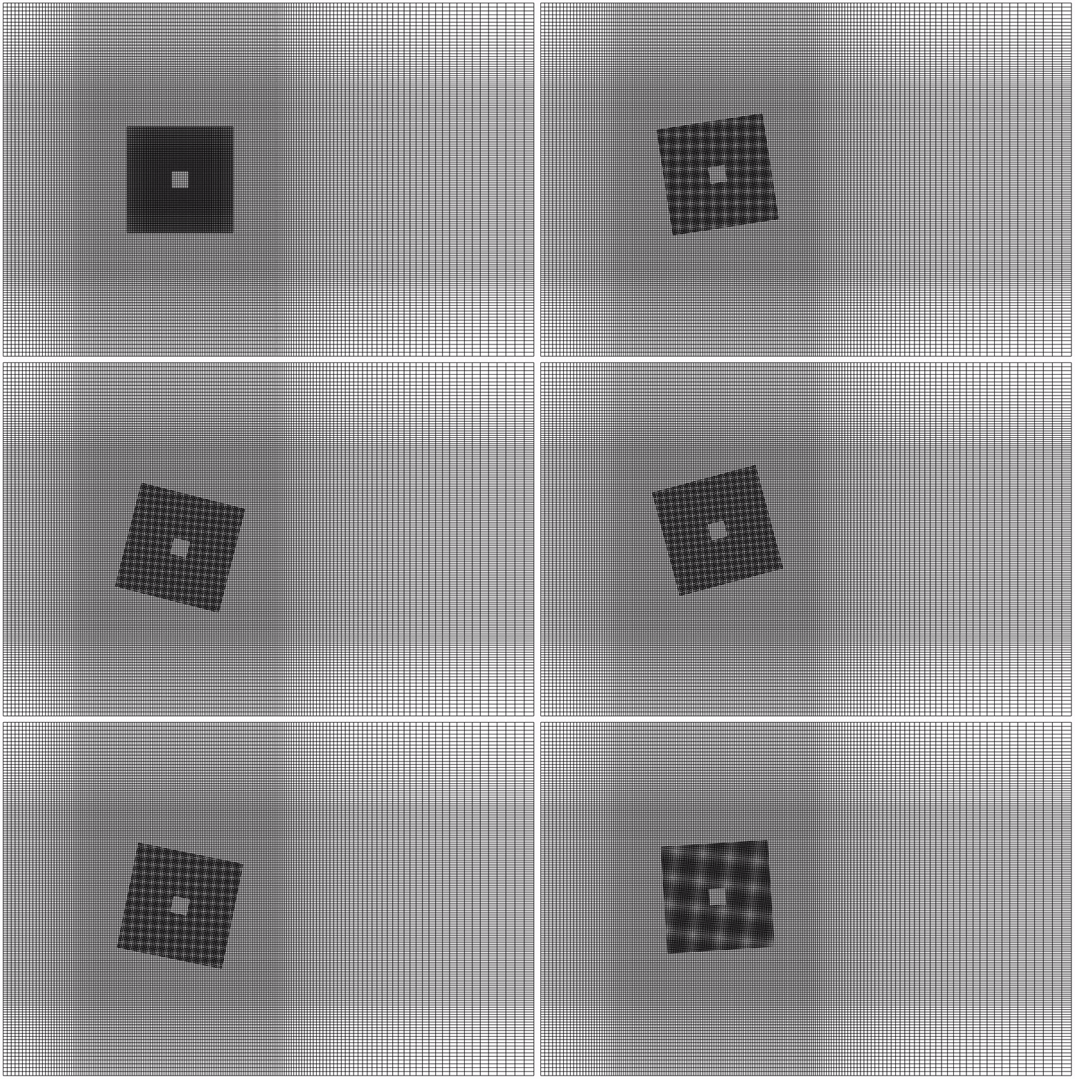
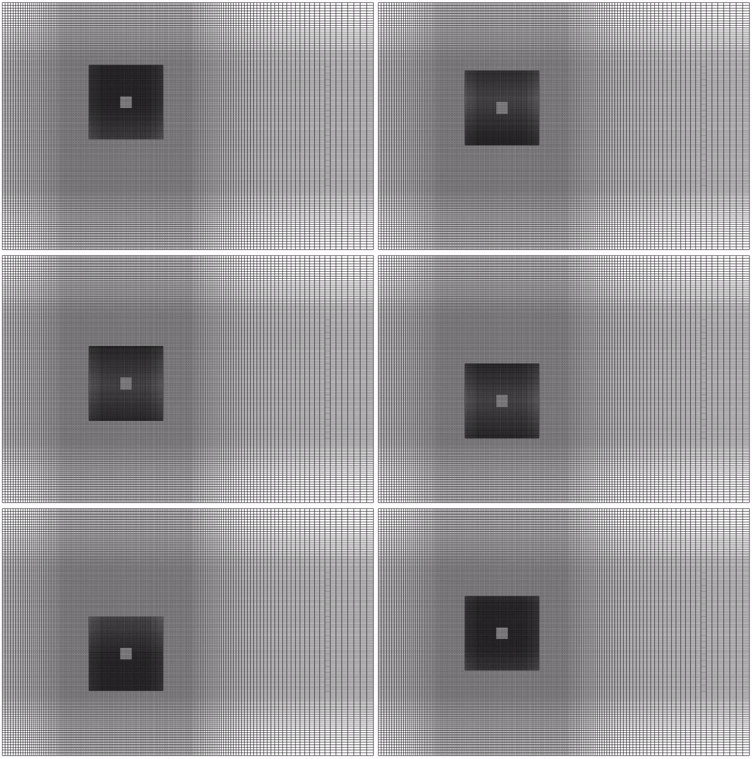
The motion we defined should look as shown below:

You can modify the heaving and pitching motion by adjusting the initial angle and phase angle accordingly.

The combination of overset mesh and tabulated6DoFMotion in OpenFOAM offers an advanced framework for simulating dynamic systems with complex motion. By enabling six degrees of freedom and accommodating pre-tabulated motion data, this approach overcomes the limitations of standard prescribed motion definitions, providing unparalleled flexibility and accuracy. From setting up overset regions to defining motion data with Python, this blog has walked through the key steps for implementing such cases.